Attention scores, Scaling and Softmax
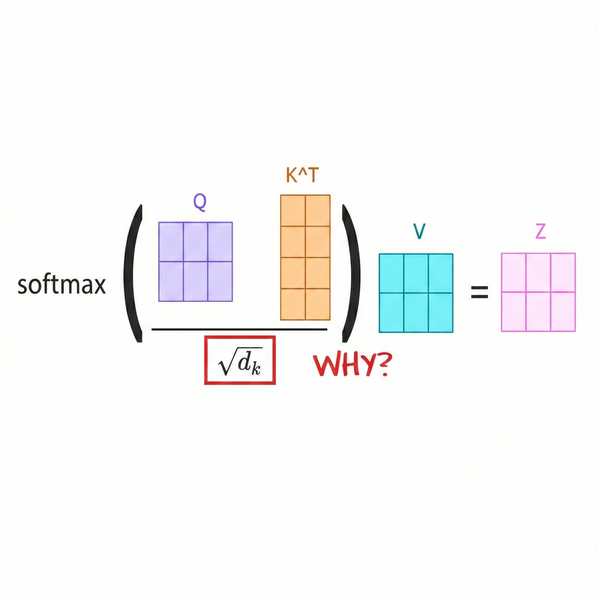
If you're familiar with the Attention Mechansim, then you know that before applying a softmax to the attention scores, we need to rescale them by a factor of $\frac{1}{\sqrt{D_k}}$ where $D_k$ is the dimension of the hidden state of the Keys parameter...but why is that?
Why should you care about these details?
Abstraction can be a powerfull concept, it allows us to build much faster: you create a self sustaining black box, and you free yourself from its burden. But can you be free from something you don’t about? In the sense that if you have a system that breaks, and you’re unaware that some abstracted parts have the ability to influence it, you’re screwed by your ignorance.
A good heuristic for me to know if something is worth investigating is a weighted combination of :
- Has the system stood the test of time?
- Do you expect it to be replaced soon?
- How much do you rely on it? Amdahl’s law
Recollection, Disection and Decomposition
If you’ve read my privous blog on the Vanishing and exploding gradient you must have a good intuition on why it’s important to keep a unit variance, and zero a mean of activations, and the Attention Mechanism doesn’t escape that.
At the core of it, whether it’s Multihead Attention or simple Attention, there’s a dot product, it’s thus of interest to us to understand what kind of properties does the results have, we will track some statistics, and see how things can go wrong, but let’s be smart about it, because the scaling is a factor of $D_k$ ($D_K$ must be equal to $D_Q$, because we’re doing matrix multplication), we can do some reverse engineering by fixing other parameters (for now :p) we can explore how changing this value effects the statistics we’re tracking.
The following code shows how we can do this manipulation:
1
2
3
4
5
6
7
8
9
10
11
12
13
14
15
16
17
18
19
20
21
22
23
24
25
26
27
28
29
30
31
32
33
34
35
36
37
38
39
import torch
import matplotlib.pyplot as plt

# Set random seed for reproducibility
torch.manual_seed(0)

# Set parameters for testing
seq_len = 512  # Number of random vectors to generate for averaging
dims = [10, 50, 100, 500, 1000]  # Various dimensions to test
variance_results = {}

for d in dims:
    # Generate random vectors with mean 0 and variance 1
    Q = torch.randn(seq_len, d)
    K = torch.randn(seq_len, d)

    # Compute dot products
    dot_products = torch.matmul(Q, K.T)

    # Calculate mean and variance of dot products for each row
    mean = dot_products.mean(dim=1)
    variance = dot_products.var(dim=1)

    # Store the mean and variance statistics
    variance_results[d] = {
        'mean': mean.mean().item(),
        'variance': variance.mean().item()
    }

# Plot the results
fig, ax1  = plt.subplots(1, 1, figsize=(12, 5))

ax1.plot(list(variance_results.keys()), [variance_results[d]['mean'] for d in variance_results], label='Mean')
ax1.plot(list(variance_results.keys()), [variance_results[d]['variance'] for d in variance_results], label='Variance')
ax1.set_xlabel('Dimensionality')
ax1.set_ylabel('Value')
ax1.set_title('Mean and Variance of Dot Products')
ax1.legend()
plt.show()
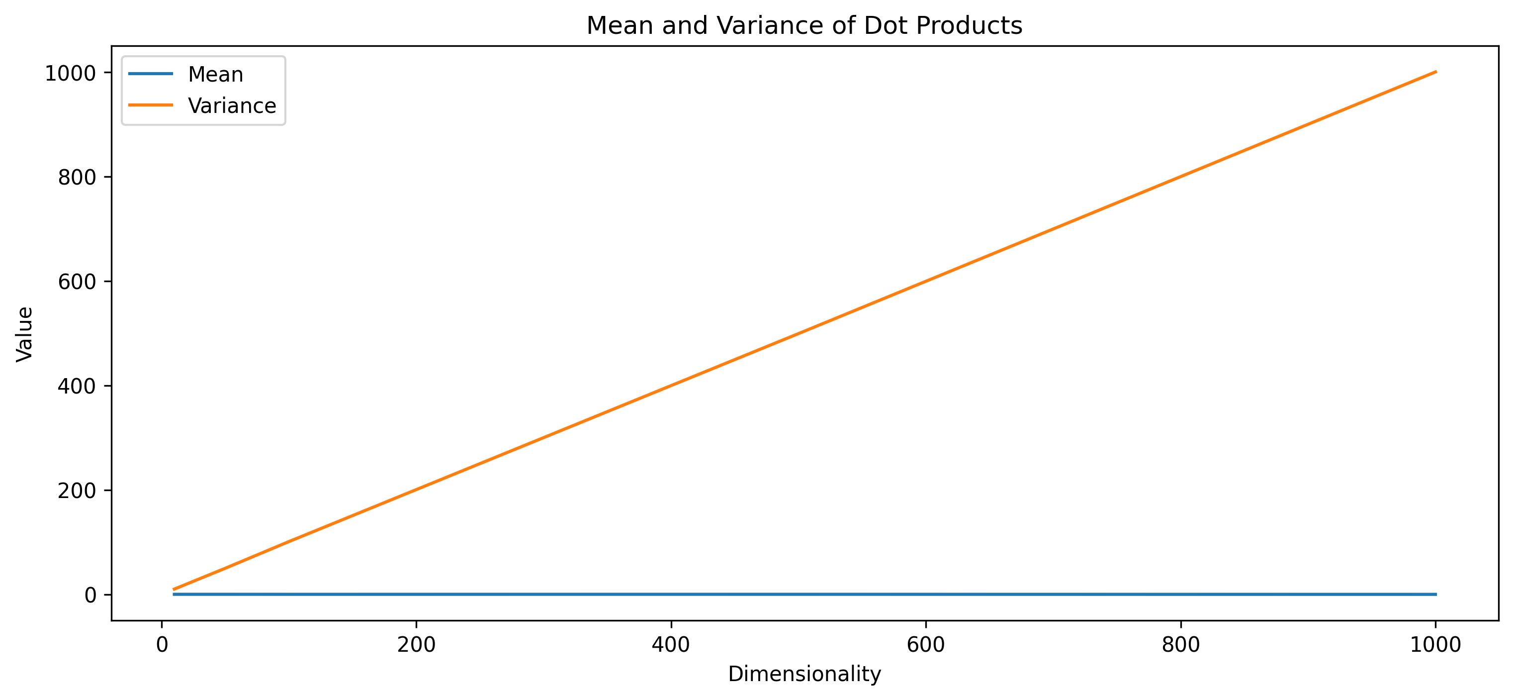
The result is striking! while the mean remains close to zero, the variance seems to increase with respect to the size of the hidden size! this is clearly not good.
The why behind the what
Let’s go through a proof of why the mean of the dot products remains the same while the variance scales linearly with dimension $ d $.
To do this, let’s define the following:
- Setup of Random Vectors: Let $ Q = [Q_1, Q_2, \dots, Q_d] $ and $ K = [K_1, K_2, \dots, K_d] $ be two vectors of dimension $ d $.
- Dot Product: The dot product of $ Q $ and $ K $ is given by:
\(Q \cdot K = \sum_{i=1}^d Q_i K_i\) where each $ Q_i $ and $ K_i $ is sampled independently from a standard normal distribution with mean $ 0 $ and variance $ 1 $.
The Mean of the Dot Product
We want to find $ \mathbb{E}[Q \cdot K ]$, the expected value of the dot product.
Expanding the Expectation
Since the dot product $ Q \cdot K $ is a sum, we can use the linearity of expectation: \(\begin{equation} \mathbb{E}[Q \cdot K] = \mathbb{E}\left[\sum_{i=1}^d Q_i K_i\right] = \sum_{i=1}^d \mathbb{E}[Q_i K_i] \end{equation}\)
Computing $ \mathbb{E}[Q_i K_i] $
Since each $ Q_i $ and $ K_i $ is an independent standard normal random variable (mean $ 0 $), variance $ 1 $, we know:
- $ \mathbb{E}[Q_i] = 0 $ and $ \mathbb{E}[K_i] = 0 $.
Therefore, the expectation of the product $ Q_i K_i $ is:
\[\mathbb{E}[Q_i K_i] = \mathbb{E}[Q_i] \cdot \mathbb{E}[K_i] = 0 \cdot 0 = 0\]
Since each term $ \mathbb{E}[Q_i K_i] = 0 $, we have:
\[\mathbb{E}[Q \cdot K] = \sum_{i=1}^d 0 = 0\]Thus, the mean of the dot product $ Q \cdot K $ is 0, regardless of the dimension $ d $.
Variance of the Dot Product
Now we want to find the variance $ \text{Var}(Q \cdot K) $ of the dot product. Recall that the variance of a sum of independent random variables is the sum of their variances:
\[\text{Var}\left(Q \cdot K\right) = \text{Var}\left(\sum_{i=1}^d Q_i K_i\right) = \sum_{i=1}^d \text{Var}(Q_i K_i)\]Computing $ \text{Var}(Q_i K_i) $
Since \(Q_i\) and \(K_i\) are independent standard normal random variables:
- Each $ Q_i $ and $ K_i $ has variance $ 1 $.
- For independent random variables, the variance of the product $ Q_i K_i $ is given by:
Since each term $ \text{Var}(Q_i K_i) = 1 $, the total variance is:
\[\text{Var}(Q \cdot K) = \sum_{i=1}^d 1 = d\]Thus, the variance of the dot product $ Q \cdot K $ is $ d $, which increases linearly with the dimension $ d $, so we defintely need to do something about it!
The Variance Condition
We know from previous calculations that:
\(\text{Var}(Q \cdot K) = d\) where $ d $ is the dimension of the vectors $ Q $ and $ K $.
We want to scale this dot product by a factor $ Z $ so that the resulting variance becomes $ 1 $. This means we are looking for a constant $ Z $ such that:
\[\text{Var}(Z \cdot Q \cdot K) = 1\]If we multiply a random variable by a constant $ Z $, the variance scales by $ Z^2 $.
Therefore:
\[\text{Var}(Z \cdot Q \cdot K) = Z^2 \cdot \text{Var}(Q \cdot K)\]Substituting $ \text{Var}(Q \cdot K) = d $ into the equation, we get:
\[\text{Var}(Z \cdot Q \cdot K) = Z^2 \cdot d\]Now, we set $ Z^2 \cdot d = 1 $ to satisfy the condition that $ \text{Var}(Z \cdot Q \cdot K) = 1 $.
Solving for $ Z $, we get:
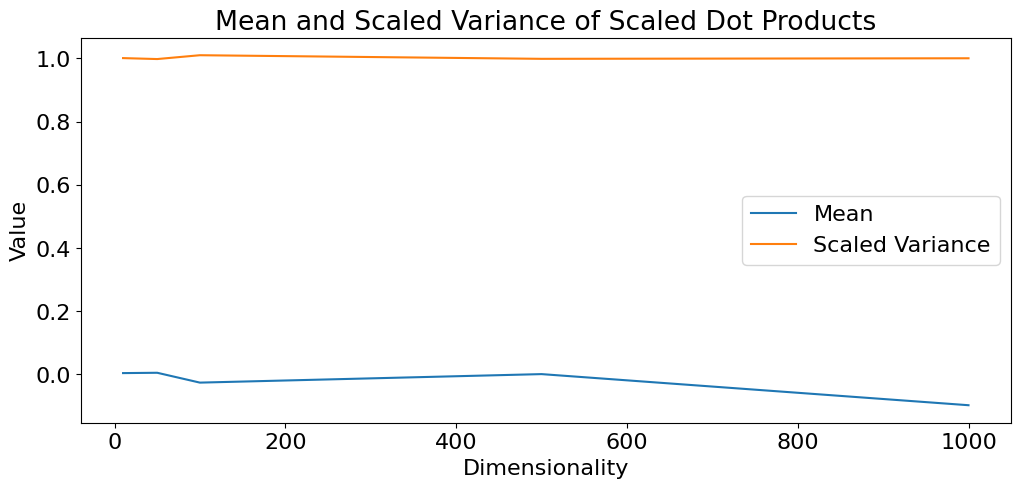
\[Z^2 = \frac{1}{d}\] \[Z = \frac{1}{\sqrt{d}}\]This is why we scale the dot product by $ \frac{1}{\sqrt{d}} $ in the attention mechanism. This choice of $ Z $ ensures that the variance of the scaled dot product $ \frac{Q \cdot K}{\sqrt{d}} $ remains at $ 1$, which keeps the values passed to softmax in a stable range, preventing overly large values and maintaining effective attention distributions.
Take a moment and enjoy this plot:
Softmax’s exaggeration
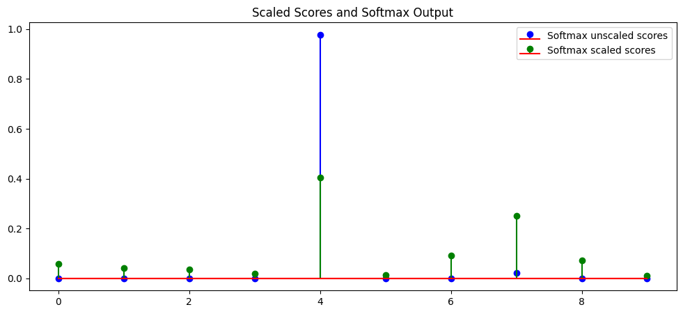
This again directly relates to the previous post on the gradients, if you have a bad distribution of the input it impacts the activations, and the softmax does not stray away from this, in fact it may even extend it, having high variance means that when applying a softmax some activation values may get extremly small/big, thus the gradient will not flow correctly through the layers, the following figure clearly showcases how scaled vs unscaled dot products behaves when applying the softmax (I like to see the effect of scaling as little push, made to give a chance to newbies).


