Do You Need A Matryoshka Model?

I recently went down a rabbit hole exploring Matryoshka Embedding Models after reading the excellent Hugging Face blog post by Tom Aarsen on the topic.

Matryoshka Representation Learning (MRL) is a neat technique that trains models to “front-load” the most critical information into the initial dimensions of an embedding. This allows you to truncate embeddings to a much smaller size with a minimal drop in performance, offering incredible efficiency gains.

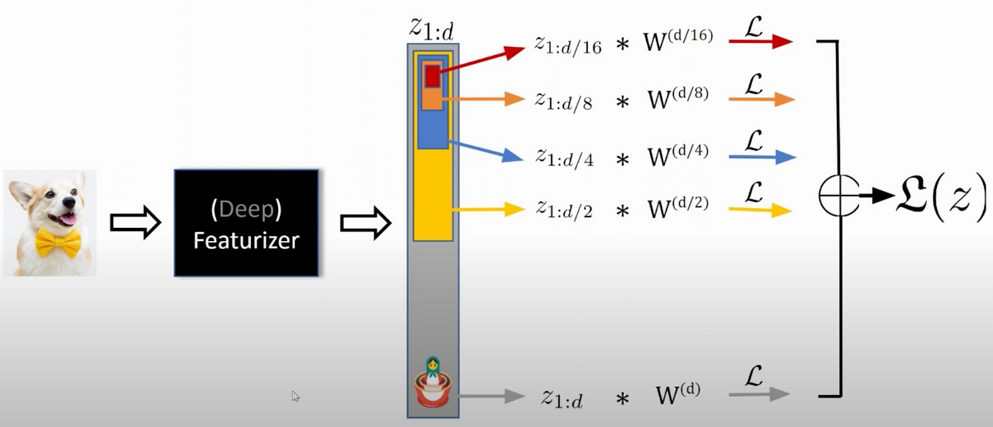Matryoshka Representation Learning

This standard approach compares a purpose-built Matryoshka model to one using what I would now call “naive truncation” (very humble of me :p yes), just taking the first k dimensions. But it sparked a question: What if the most valuable information in a standard model isn’t even at the beginning? What if its performance is concentrated elsewhere?

To investigate this, I designed an experiment to map the performance contribution of different segments within a standard sentence embedding.

Methodology

• Model: tomaarsen/mpnet-base-nli (a 768-dimension Transformer model).
• Task: Semantic Textual Similarity (STS) performance, measured by Spearman correlation on the MTEB STSBenchmark dataset.
• Technique: I used a “sliding window” approach. A 64-dimension window was moved across the entire 768-dimension embedding with a step size of 16 dimensions. This created 45 overlapping segments (0-64, 16-80, 32-96, etc.), and a full STS evaluation was run on each one.
• Generalization Check: To see if the patterns were consistent, I repeated this entire process across the train, validation, and test splits of the dataset.

Finding 1: Performance is Not Uniformly Distributed

The performance of the segments was not random. Across the test set windows, scores ranged from a low of 81.76% to a high of 84.55%, with a mean of 83.16% and a tight standard deviation of 0.57. As the following plot shows, the most performant segments are concentrated in the first half of the embedding (around 150-350), suggesting that for this model, simply truncating the first k dimensions is a suboptimal strategy.

Normalized Performance Distribution

Finding 2: This “Information Map” Generalizes Surprisingly Well

The next question was critical: is this pattern just a fluke on the test set? I ran the same experiment across the train, validation, and test splits. The result was interesting:

• Strong Generalization (Train vs. Test): The overall shape of the performance curve is remarkably consistent between the train and test sets, showing a strong correlation of 0.7872. This suggests the model has learned a robust and generalizable internal structure for which regions are important.
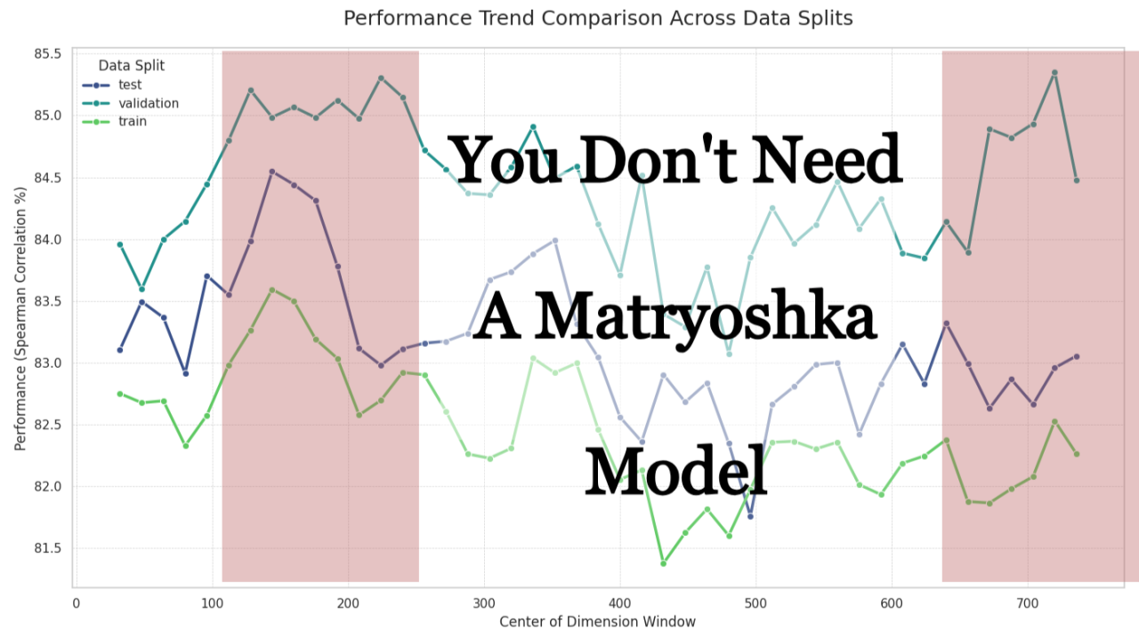
• Weaker Generalization (Validation vs. Test): The correlation between the validation and test sets was much lower at 0.4799. As next plot shows, while the broad peaks and valleys align, the fine-grained, window-to-window performance is noisy.

This suggests that while we can be confident about the general “hotspot” regions, we should be cautious about concluding that one specific 64-dimension window is definitively better than its neighbor.

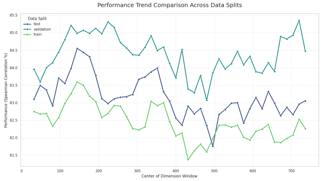Performance Trend Comparison

What is the Potential Practical Utility?

Informed Truncation: This analysis could allow us to perform “informed” truncation, selecting the most powerful (e.g., 128 or 256) dimensions, wherever they might be, to potentially maximize performance for a given embedding size.

A Hypothesis for Efficient Retrieval: This knowledge could be used to build more efficient two-stage search systems. A small but powerful segment of the embedding could be used for a fast initial candidate search, followed by a re-ranking step using the full embedding.

A New Diagnostic Tool: This “embedding cartography” offers a new way to analyze our models. It moves beyond a single metric to visualize the internal information structure, which could be invaluable for model debugging and comparison.I’m curious to hear what the community thinks. Has anyone else explored this kind of analysis? What other practical applications can you see for mapping out the performance of our models’ embeddings?

The Next Question: Structured vs. Diffuse Information

This experiment showed that contiguous blocks of dimensions have a clear structure. But this raises a new question: how essential is this contiguity ? Or is the information more diffuse, where any 64 random dimensions could perform just as well?

For those interested, I’ve open-sourced the notebook for this analysis on GitHub.

Link to the project