Elements Of Mechanistic Interpretability: From Observation to Causation
We strip down mechanistic interpretability to three key experiments: watching a model 'think', finding where it stores concepts, and performing 'causal surgery' to change its 'thought process'
During my time at Orange, I worked on evaluating how LLMs handle input perturbations in code generation contexts. The results? They’re surprisingly (or not :p) brittle. While tokenization plays a role (a compelling argument for byte-level tokenization), the deeper issue lies in how neural networks represent and transform concepts layer by layer to form predictions.
To better steer these models toward our goals, we need to understand their inner workings. Despite being called “black boxes,” recent developments in mechanistic interpretability have begun illuminating what happens inside.
My first encounter with this field was while scrolling through the Effective Altruism Forum. I remember feeling overwhelmed, retrospectively, I understand this was likely because I didn’t grasp transformer internals well enough.
So my goal here is to provide practical and visual exp lanations all by attempting to not down in the details. I’ll cover techniques that help answer:
- What is the model “thinking” as it generates a response?
- Where in its “brain” (which layers) does it store specific concepts, like grammar?
- Why did it make a specific decision? Can we prove which components are responsible?
It turns out, there are simple, powerful experiments for each.
Part 1: The Observational Toolkit - “What” and “Where”
First, we need tools to just look inside the box. Before we can form hypotheses, we need to gather data.
Experiment 1: The Logit Lens (Watching the Model “Think”)
The Question: What is the model actually thinking, layer by layer, as it’s about to make a prediction?
The “Toy Problem”: A simple, factual prompt. Let’s ask a model (like SmolLM2-360M-Instruct) a question and observe how its answer evolves.
Prompt: “A group of owls is called a”
The correct answer is “parliament”
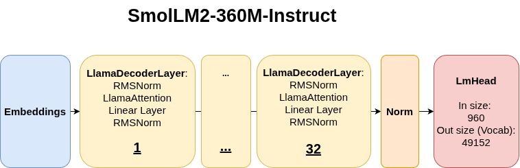 The SmolLM2-360M-Instruct Architecture: A 32-layer transformer model.”
Instead of just looking at the final prediction, we use the Logit Lens. The idea is simple: we take the hidden state at the very last token (right after “a”) from every single layer in the model. We then project each of these 32 hidden states back into the full vocabulary space to see what the model “would have said” if that layer were the last one.
Think of it like watching a student work through a math problem. Instead of only seeing their final answer, we peek at their scratch work after each step. Each layer’s hidden state is like that intermediate work. We project the hidden states through the language model head (the same weights used at the final layer) to decode what the model “has in mind” at that point.
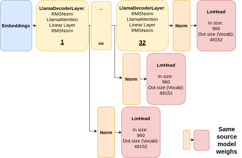 Logit Lens Mechanism: At each layer, we extract the hidden state and pass it through the final normalization and language model head to get vocabulary predictions.
Notice how I also apply normalization to the activation, without which these would be out of distribution with respect to LmHead, and the prediction would be gibberish.
The result is that we can literally watch the model’s “thought process” unfold across layers:
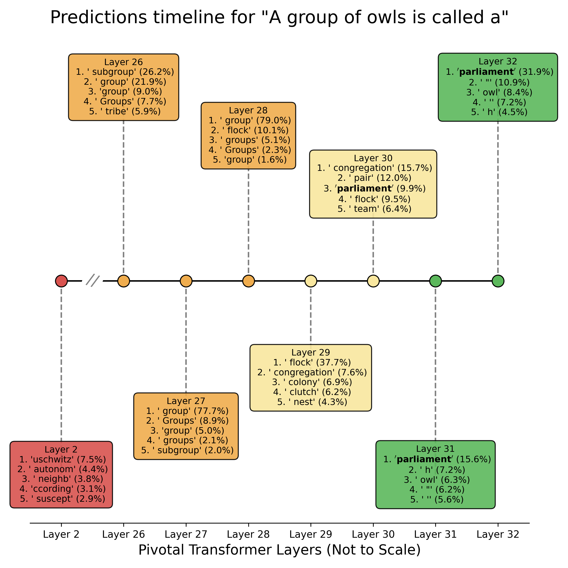 Layer-by-Layer Prediction Evolution: Each box shows the top 5 predicted tokens and their probabilities when projecting that layer’s hidden state through the language model head. Notice how “parliament” only becomes the top prediction in the final layers.
Looking at the timeline visualization:
Layer 2 (Early processing): The model is almost random, suggesting tokens like ‘uschwitz’, ‘autonom’, ‘neighb’. Clearly no coherent understanding yet, although ‘neighb’ might be hinting at what’s happening. The hidden states are still processing raw token information.
Layers 26-28 (Middle layers): Generic collective nouns emerge: ‘group’ dominates at 77-79%, alongside ‘Groups’ and ‘subgroup’. The model grasps we’re talking about collections but hasn’t retrieved specific knowledge yet.
Layer 29 (Knowledge retrieval begins): Here ‘flock’ jumps to 37.7%, showing bird-specific knowledge activating. Other bird-related terms appear: ‘congregation’, ‘colony’, ‘clutch’, ‘nest’.
Layers 30-32 (Refinement and convergence): The specific answer crystallizes: ‘parliament’ climbs from 9.9% → 15.6% → 31.9%, decisively winning by the final layer. The model has successfully retrieved the precise collective noun for owls.
Notice the progression: random → generic (group) → domain-specific (flock) → precise (parliament).
The Logit Lens works by applying the final layer’s unembedding matrix (LmHead) to hidden states from intermediate layers. This assumes the model maintains representations in a space where this projection produces meaningful results, essentially, that all layers are working toward the same vocabulary space. This is a useful but imperfect assumption, as early layers may encode information quite differently than late layers.
The Logit Lens gives us a “live feed” of the model’s layer-by-layer reasoning, confirming that knowledge isn’t stored in one place but is progressively refined through the network’s depth.
But this raises a deeper question: we can see what the model is thinking, but where exactly are specific concepts (grammar rules, factual knowledge, or semantic relationships) actually stored? Which layers specialize in which types of information? That’s where our next experiment comes in…
Experiment 2: Probing Classifiers (Finding Where Concepts Live)
The Question: Where in the network does the model represent specific linguistic concepts? Do early layers handle syntax while later layers handle semantics?
The “Toy Problem”: Let’s test something fundamental: Part-of-Speech (POS) tags. Specifically, can we distinguish between nouns and verbs just by looking at a layer’s internal representation?
The Setup
The idea behind probing is elegantly simple: if a layer’s hidden states contain information about a concept (like whether a word is a noun or verb), we should be able to train a simple classifier to extract that information.
Importantly we’re not training the language model itself (we freeze it completely). We only train a tiny “probe” (a simple linear classifier) on top of each layer’s activations. We must train a separate, independent probe for each layer, as the vector representations at layer 5 might exist in a completely different geometric space than those at layer 20. If this simple probe can accurately classify the concept, that means the information was already present in that layer’s representation.
A common pitfall in probing is asking: are we measuring what’s encoded in the activations, or what a small classifier can learn from scratch? This is why we use Linear probes and not MLPs. Simple classifiers are less likely to learn the task themselves, especially when combined with regularization (like weight_decay=0.01 in AdamW).
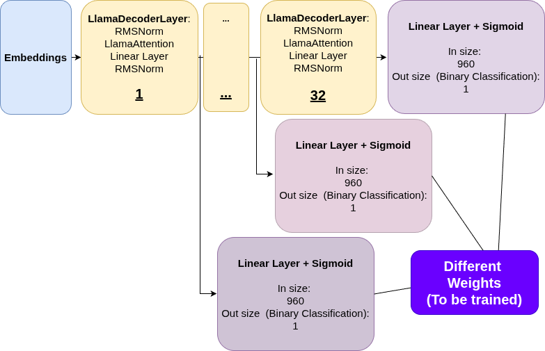 The architecture for probing classifiers. Hidden states are extracted from each transformer layer (e.g., Layer 1, Layer 32) and fed into a separate simple classifier (a Linear Layer + Sigmoid for binary classification).
I used 5,000 sentences from the SST-2 sentiment dataset, processed them with SpaCy to identify nouns and verbs, then extracted the corresponding hidden states from SmolLM2-360M-Instruct.
We could end up with a probe achieving 85% accuracy and declare victory. But what does 85% actually mean? Is the model encoding genuine linguistic structure, or are we just picking up on spurious correlations?
To answer this, we have to implement a three control experiments:
- Shuffled Labels: Train probes on the same activations but with randomly shuffled labels. This tests if we’re just memorizing noise.
- Random Embeddings: Replace the real activations with random vectors of the same dimension. This establishes a floor baseline.
- Majority Class Baseline: Always predict the most common class (in this case, nouns at ~69%).
(I also trained with 5 different random seeds to measure variance and ensure reproducibility.)
The Results: A Clear Story Emerges
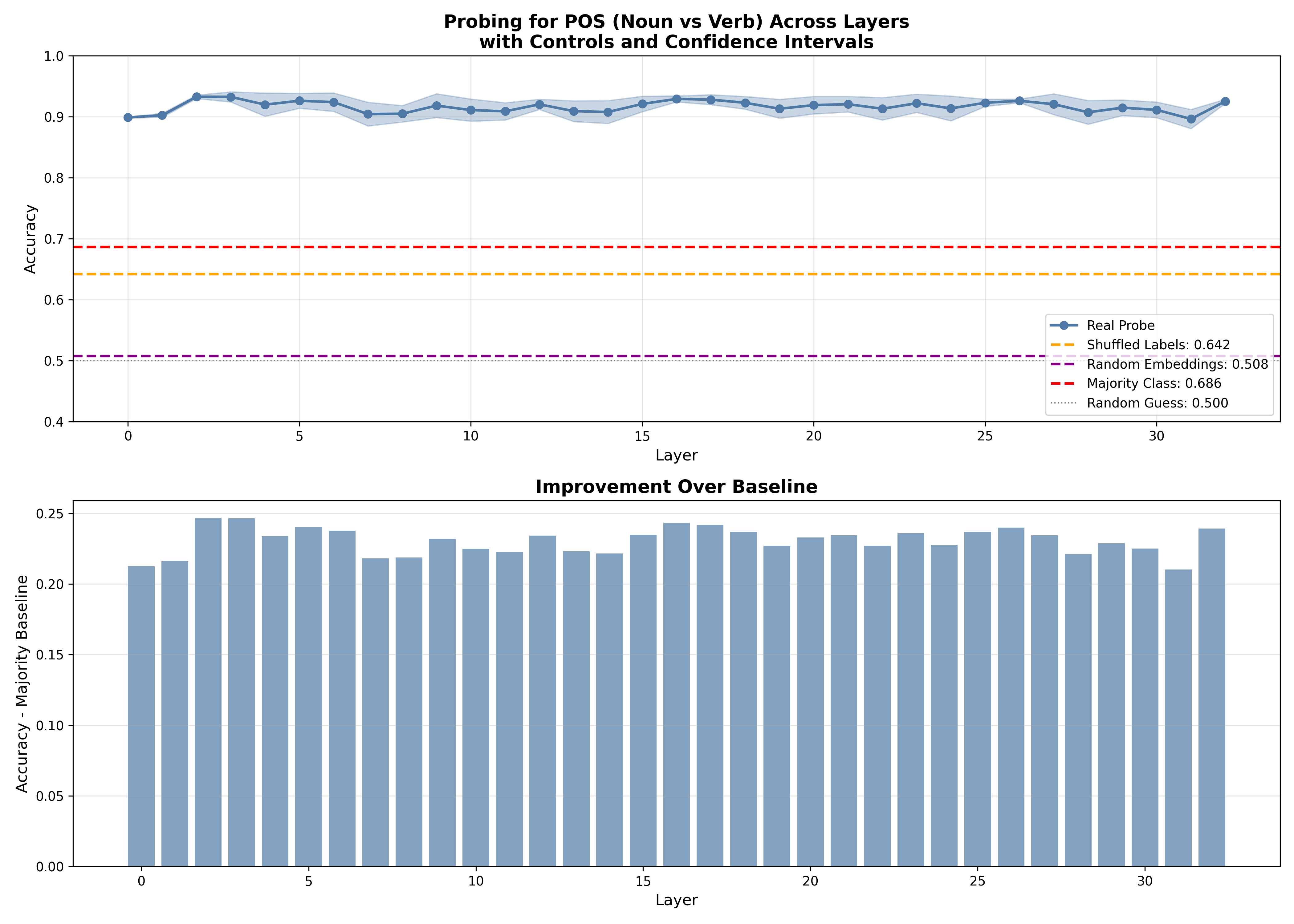
The graph reveals several striking patterns:
1. High baseline performance everywhere (~90-93% across all layers)
- This immediately tells us something important: POS information is encoded everywhere in the network, from the very first embedding layer onwards.
- Even the embedding layer (layer 0), which only knows about individual tokens without any context, achieves ~90% accuracy.
2. Slight peak in early-to-middle layers (layers 2-4)
- We see a small bump to ~93% in layers 2-4, suggesting these layers are refining syntactic representations.
- This aligns with the intuition that early layers should handle syntax.
3. Remarkably flat performance
- Unlike some other probing tasks, POS tagging doesn’t show dramatic differences between layers.
- The improvement over the majority baseline is consistent (~23-25 percentage points) across the network.
4. Controls confirm genuine learning
- Shuffled labels: ~64% (barely above random)
- Random embeddings: ~51% (essentially random guessing)
- Majority class: ~69%
All controls fall well below the real probes, confirming we’re not just fitting noise.
What This Tells Us
The flatness of the curve is itself informative. Unlike semantic tasks (which might require deeper layers to resolve), basic syntactic category is:
- Partially encoded in the vocabulary (layer 0 already knows common nouns vs. verbs)
- Refined with minimal context (early layers add a small boost)
- Preserved throughout the network (later layers don’t degrade this information)
This makes sense: knowing whether “bank” is a noun or verb is fundamental to sentence processing, so the model maintains this information everywhere rather than computing it once and discarding it.
The Hard Test: Homographs
But here’s the real question: can the model handle context-dependent POS tagging? Words like “watch,” “book,” and “play” can be both nouns and verbs. The model needs to use context to disambiguate.
A homograph is a word that is spelled the same as another word but has a different meaning and may have a different pronunciation.
I tested 5 homograph pairs on out-of-distribution sentences, here are 2 of them:
1
2
3
4
5
6
7
8
9
10
11
12
13
14
15
Word: 'watch'
  NOUN: "He bought a new watch."
  VERB: "They watch movies every night."

Layer    P(Noun|NOUN ctx)   P(Noun|VERB ctx)   Both Correct?
------   -----------------  -----------------  -------------
Embed         0.060 ✗            0.060 ✓             ✗
L5            0.933 ✓            0.001 ✓             ✓
L10           1.000 ✓            0.000 ✓             ✓
L15           0.951 ✓            0.002 ✓             ✓
L20           1.000 ✓            0.004 ✓             ✓
L25           1.000 ✓            0.000 ✓             ✓
L30           1.000 ✓            0.000 ✓             ✓
L32           1.000 ✓            0.012 ✓             ✓
And
1
2
3
4
5
6
7
8
9
10
11
12
13
14
Word: 'book'
  NOUN: "She put the book on the table."
  VERB: "Please book our flight."

Layer    P(Noun|NOUN ctx)   P(Noun|VERB ctx)   Both Correct?
------   -----------------  -----------------  -------------
Embed         0.950 ✓            0.950 ✗             ✗
L5            0.999 ✓            0.002 ✓             ✓
L10           1.000 ✓            0.016 ✓             ✓
L15           0.999 ✓            0.007 ✓             ✓
L20           1.000 ✓            0.101 ✓             ✓
L25           1.000 ✓            0.265 ✓             ✓
L30           1.000 ✓            0.660 ✗             ✗
L32           0.991 ✓            0.253 ✓             ✓
Key observations:
1. The embedding layer reveals lexical priors, not context Notice how the embedding layer gives identical probabilities for the same word in both contexts:
- “watch”: 0.060 in both (strongly predicts verb - “watch” is usually a verb in training data)
- “book”: 0.950 in both (strongly predicts noun - “book” is usually a noun)
This makes perfect sense: at layer 0, we only have the token embedding as no attention has happened yet, so there’s no way to incorporate context. The probe is simply learning which words tend to be nouns vs verbs in general.
2. Context-dependent disambiguation emerges by layer 5
By layer 5, the model has processed attention and can use surrounding words:
- For “watch”: noun context → 0.933, verb context → 0.001 (near-perfect separation!)
- For “book”: noun context → 0.999, verb context → 0.002
The attention mechanism has successfully used words like “bought” vs “They…movies” to resolve the ambiguity
3. Later layers maintain strong performance with some interesting exceptions
Most homographs remain correctly classified through layer 32 with the exception of “book as a verb” which becomes harder for layers 30-32 (drops to 0.660 confidence in noun class)
This suggests that later layers might be doing something more complex than just preserving syntactic information
Implications for Interpretability
Probing teaches us several lessons:
Information is distributed: Concepts aren’t stored in a single “POS neuron”, instead they’re encoded across the entire representation space.
Layer specialization is subtle: Unlike the clean story some papers tell (“early layers = syntax, late layers = semantics”), real networks show more nuanced patterns.
Context processing happens gradually: Even “simple” tasks like POS tagging require multiple layers to handle ambiguous cases.
But here’s what probing doesn’t tell us: correlation ≠ causation. We’ve shown that POS information exists in layer 15, but does the model actually use that representation to make predictions? Or is it just a vestigial side effect of training?
To answer this causal question, we need a different kind of experiment entirely…
Part 2: From Observation to Causation - “Why”
Probing told us where information lives. Now we need to prove which components matter for the model’s decisions.
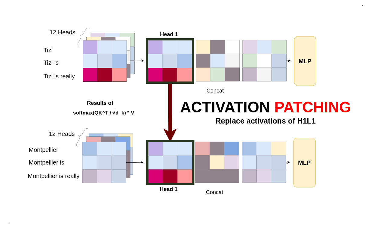
Experiment 3: Activation Patching (Causal Surgery)
The Question: Which specific attention heads are causally responsible for the model’s behavior? Can we prove that a particular head is critical to a task?
The “Toy Problem”: A more structured task called Indirect Object Identification (IOI). Given a sentence like:
“When Jack and Harry went to the store, Jack gave a book to ___”
The model should predict “Harry” (the indirect object who isn’t Jack). This requires:
- Identifying both names (Jack, Harry)
- Recognizing Jack is the subject
- Retrieving “the other name” (Harry) as the answer
This is perfect for causal analysis because we can create minimal pairs:
- Clean prompt: “When Jack and Harry went to the store, Jack gave a book to” → should predict Harry
- Corrupted prompt: “When Ron and Wiz went to the store, Ron gave a book to” → should predict Wiz
For this experiment, I’m using GPT-2 Small, which has a more manageable architecture to analyze:
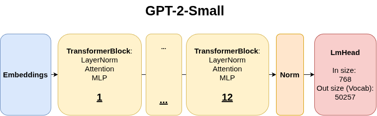 GPT-2 Small Architecture: 12 layers, each with 12 attention heads, for a total of 144 attention heads to investigate. Each head processes information independently before results are combined.
The Technique: Activation Patching
Here’s the brilliant idea: What if we could perform “surgery” on the model’s forward pass?
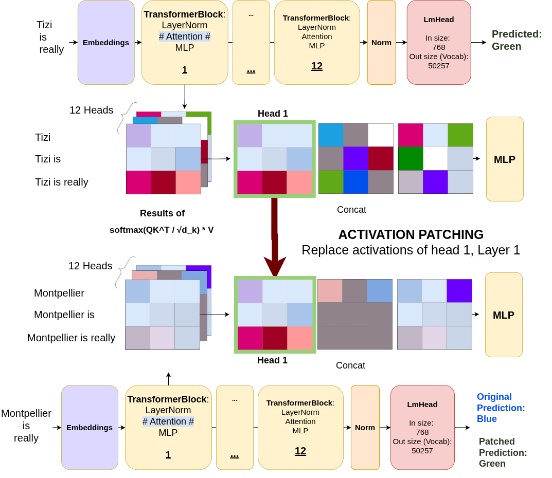 Activation Patching Setup: We run two forward passes (clean and corrupted) and selectively replace activations from specific components in the corrupted run with their clean counterparts. If replacing a head’s activation restores the correct prediction, that head was causally important.
The procedure:
- Run the clean prompt (Jack/Harry) through the model and cache all activations
- Run the corrupted prompt (Ron/Wiz) normally - it predicts “Wiz”
- For each attention head individually:
- Run the corrupted prompt again
- But this time, replace that head’s output with its cached activation from the clean run
- Measure: did the prediction shift toward “Harry”?
- Repeat for all 144 heads (12 layers × 12 heads in GPT-2)
If patching a head makes the model suddenly prefer “Harry” over “Wiz”, we’ve found a causal component - that head was responsible for retrieving the correct indirect object.
The Metric: Logit Difference
We measure the model’s preference using logit difference:
1
Logit Diff = logit("Harry") - logit("Wiz")
- Clean run: Large positive value (~12.13) → strongly prefers Harry
- Corrupted run: Negative value (~-2.62) → strongly prefers Wiz
- After patching: If logit diff increases, that head helped retrieve the correct name
The Results: Finding the “Name Mover Heads”
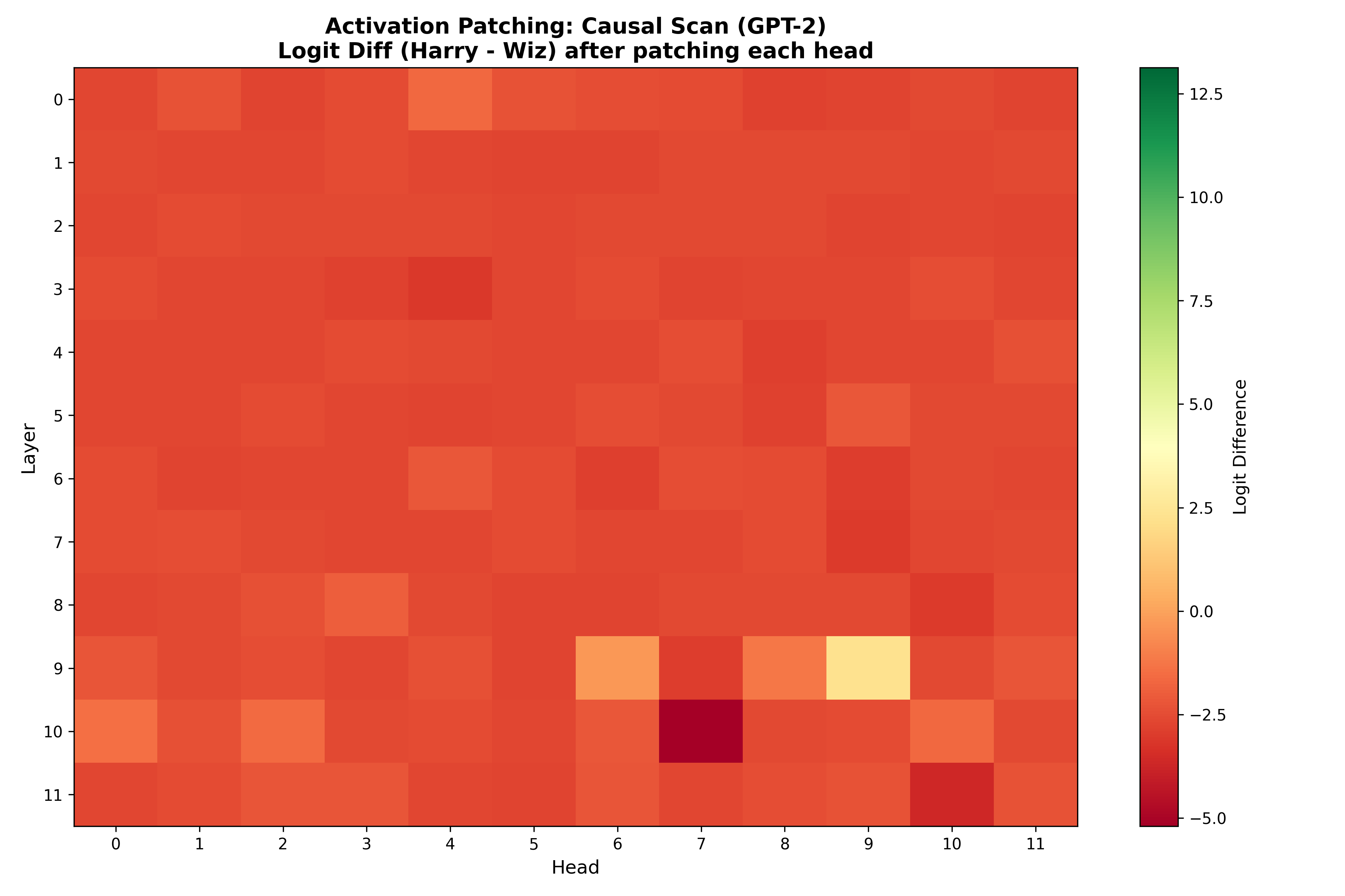 Causal Discovery Heatmap: Each cell shows the logit difference after patching that specific head. Green = helps restore “Harry”, Red = maintains “Wiz”. Most heads have little effect, but L9H9 is the clear standout.
The heatmap is clearly showing that the vast majority of the 144 heads cluster around the corrupted baseline (~-2.62). Patching them has minimal effect. This tells us something profound: most of the network’s computation is not causally relevant to this specific task.
One head dominates - Looking at layer 9, we see L9H9 stands out dramatically as togit diff jumps to +2.26 (a swing of ~5 logits from the corrupted baseline!); L9H6 shows effect but much weaker than L9H9; all other heads essentially have a simliar upshot from the baseline.
L9H9 is the “Name Mover Head” : a single attention head primarily responsible for retrieving the indirect object name.
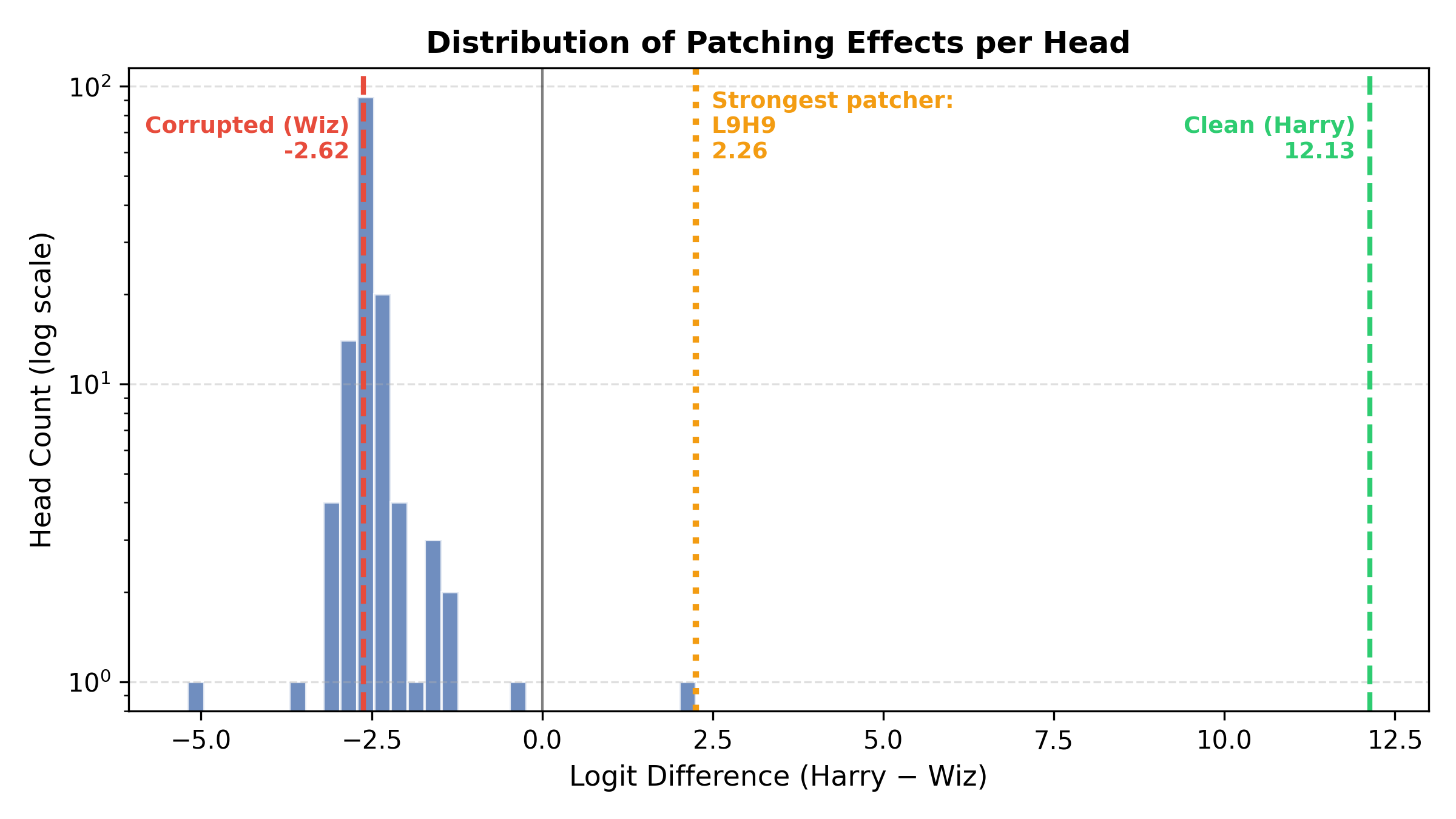 Distribution of Patching Effects: A log-scale histogram showing that causal heads are extremely rare outliers. L9H9 sits at +2.26, nearly 5 logits away from the corrupted baseline (-2.62), while the vast majority of heads cluster tightly around the baseline with minimal effect.
This is the power of activation patching: we’ve moved from “POS information exists everywhere” (probing) to “this one specific head causes most of the indirect object behavior” (causation).
What Makes a “Name Mover Head”?
Now let’s dig deeper into what L9H9 is actually doing. The attention pattern reveals the mechanism:
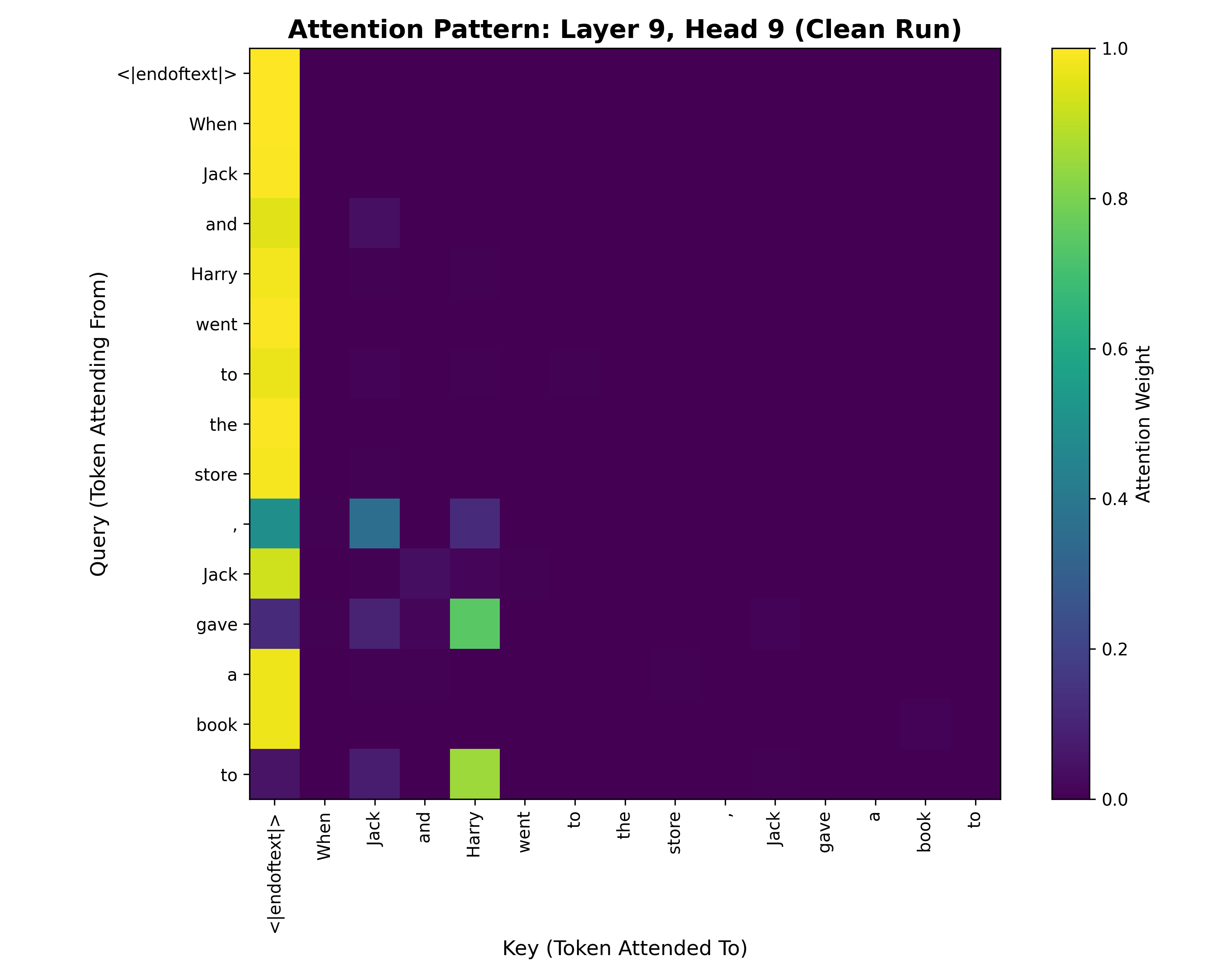 Attention Pattern of L9H9 on Clean Prompt: Rows show query tokens (where attention originates), columns show key tokens (what gets attended to). The critical row is
 <|endoftext|> (the final position where we predict the next token).
<|endoftext|>in gpt-2 also behaves like a beginning of sequence token (bos), which is what it’s referring to in the image
Looking at the bottom row (“to” - our prediction position), we see this head attends slightly to itself (“to” token) and to “Jack” (first occurrence). But what’s crucial is that it attends heavily to the “Harry” token.
This is exactly what we mean by a name mover head - it literally moves name information from where it appears in the sentence to where it’s needed for the prediction.
Conclusion: Opening the Black Box
Mechanistic interpretability gives us tools to look inside neural networks and understand their internal mechanisms. The three techniques covered here form a practical toolkit:
- Logit Lens: Observe how predictions evolve across layers
- Probing: Locate where concepts are represented
- Activation Patching: Prove which components are causally important
These aren’t just theoretical exercises. They reveal how transformers actually work: knowledge is progressively refined through layers, information is distributed across representations, and behavior emerges from sparse, specialized sub-circuits.
The field is still developing, and many questions remain open. But we now have concrete methods to investigate model internals, rather than treating them as inscrutable black boxes.
Where to Go From Here
All experiments are available at github.com/MostHumble/mech-interp-cookbook
For further reading:
- (Mechansitic Interpretability course)[https://arena-chapter1-transformer-interp.streamlit.app/] by Callum McDougall et al.
- The IOI paper (Wang et al.) - comprehensive circuit analysis
- Anthropic’s circuits work - beautiful visualizations and deep dives
- The Logit Lens post (nostalgebraist) - original technique
- TransformerLens documentation - library for mechanistic interpretability, which I used for the activation patching part.