SFT vs. DPO (/ RLHF)- A Visual Guide to What Your LLM Actually Learns

I’ve always found the best way to grasp a complex machine learning concept is to strip it down to a simple, visual experiment. Recently, I wanted to build a better intuition for the difference between Supervised Fine-Tuning (SFT) and alignment techniques like Direct Preference Optimization (DPO). We often hear that SFT is for imitation and DPO is for optimization, but what does that look like in practice?

To find out, I designed a toy problem that’s easy to understand, quick to reproduce, and visually compelling. My goal was to create a clear, undeniable demonstration of how these two powerful fine-tuning methods lead a model to learn fundamentally different behaviors.

The Toy Problem: A Grammar of Colored Tiles

Let’s imagine a simple world with only three colored tiles: Red (R), Green (G), and Blue (B). You can create sequences of these tiles, but you have to follow a strict grammar:

• Red (R) must be followed by Green (G).
• Green (G) must be followed by Blue (B).
• Blue (B) can be followed by either Red (R) or Green (G).

These are the local rules. But there’s also a global objective: we want to create sequences with the highest possible “preference score,” which we’ll define as the frequency of the B -> G transition. This transition is the only point of choice in our grammar, and mastering it is the key to achieving our goal.

The challenge for our language model is two-fold:

1. Learn the Grammar: Generate sequences that are syntactically valid.
2. Maximize the Preference: Learn to favor the B -> G transition over B -> R to achieve a higher score.

The Experimental Setup: Models, Metrics, and Data

Before diving into the training, let’s quickly cover the core components of the experiment.

The Model and Tokenizer

To keep things simple and fast, I trained a small GPT-2 model from scratch. It has just 6 layers, 4 attention heads, and an embedding size of 256, resulting in a model with about 4.8 million parameters. This is tiny by modern standards, but perfect for a controlled toy problem.

More importantly, I created a custom character-level tokenizer. Since our world only contains ‘R’, ‘G’, and ‘B’, using a standard tokenizer would be inefficient. A simple character tokenizer ensures a perfect, one-to-one mapping between our vocabulary and the model’s understanding, giving us a clean, controlled environment.

The Evaluation Metrics

To measure success, I used three key metrics:

1. Preference Score: This is our primary objective, measuring the frequency of the preferred B -> G transition in a generated sequence.
2. Rule Adherence: This is a sanity check that measures the percentage of valid transitions in a sequence. A high score means the model hasn’t forgotten its pre-training.
3. Output Entropy: This metric serves as a proxy for creativity or variety. A higher entropy means the model produces a wider range of different sequences, while a lower entropy suggests it has converged on a smaller set of preferred outputs.

Generating the Training Data

The entire experiment hinges on creating distinct datasets for each stage. For pre-training, we simply need a large corpus of grammatically correct sequences (20k) to teach the model the rules of our world.

For SFT and DPO, the data generation is more nuanced. The process begins by generating a random, valid sequence of tiles to act as a prompt (which sequence lengths go from 1 through 20). Then, two different valid continuations (completions until 40 tokens) are generated from that same prompt. By calculating the preference score for both resulting sequences, we can label one completion as “chosen” (the winner) and the other as “rejected” (the loser). This creates the (prompt, chosen, rejected) triplets needed for DPO. For the SFT dataset, we simply take the best (prompt, chosen) pairs, ensuring both fine-tuning methods are trained on the same underlying preference data.

(side note: if you do the math 40 tokens here means 140k possibilities)

The Training Pipeline: From Linguist to Apprentice

With our setup defined, we can move on to the training.

Stage 1: Pre-training (The Linguist)

Using the pre-training data, I trained our small GPT-2 model. This gives us a BASE model that can produce grammatically correct sequences but has no concept of our “preference” for B -> G transitions.

Stage 2: Fine-Tuning (Two Philosophies)

Next, I took the pre-trained BASE model and fine-tuned it using our two competing strategies:

1. The SFT Model (The Imitator) The SFT model was trained on the curated dataset of the best “chosen” completions. Its objective is to minimize the standard cross-entropy loss.

\[\mathcal{L}_{\text{SFT}}(\theta) = -\mathbb{E}_{(x, y) \in \mathcal{D}} \left[ \sum_{t=1}^{|y|} \log p_{\theta}(y_t | x, y_{<t}) \right]\]

In this equation, the model tries to maximize the log-probability of predicting the correct next token ŷ (R, G or B) for every position in the example sequences (y) from our curated dataset (D), given the prompt x (A sequence of Rs, Gs, and Bs)

An inference example

2. The DPO Model (The Explorer) The DPO model was trained on the preference pairs. Instead of just imitating, it learns an internal reward system to understand why one sequence is better than another.

The DPO loss function is where the magic happens:

\[\mathcal{L}_{\text{DPO}}(\pi_\theta; \pi_{\text{ref}}) = -\mathbb{E}_{(x, y_w, y_l) \sim \mathcal{D}} \left[ \log \sigma \left( \beta \log \frac{\pi_\theta(y_w|x)}{\pi_{\text{ref}}(y_w|x)} - \beta \log \frac{\pi_\theta(y_l|x)}{\pi_{\text{ref}}(y_l|x)} \right) \right]\]

Let’s break that down:

• $ \pi_\theta $ is our policy model that we’re training.
• $ \pi_{\text{ref}} $ the original, frozen BASE model.
• $x$ represents the prompt, in the toy example I generated rule adhering sequences of lenghts 1 to 20.
• $y_w$ and $y_l$ are the “winner” and “loser” completions from our preference pair (B->G defined as better than B->R), the max sequence lenght is 40 tokens

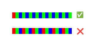Preference example

• The core of the formula measures how much more likely our new model is to generate the winning response compared to the original model.
• The loss function works by maximizing this likelihood ratio for the winning response while minimizing it for the losing response. The $\beta$ parameter acts as a regularization term, controlling how far our new model can stray from the original one.

The Results: When Imitation Isn’t Enough

After training, I had each model generate 200 sequences of 40 tokens and analyzed their performance. The results were incredibly clear.

Model	Avg. Preference Score	Avg. Rule Adherence	Output Entropy (Variety)
BASE	0.2434	86.66%	7.64 bits
SFT (Imitator)	0.2966	92.62%	7.64 bits
DPO (Explorer)	0.4551	88.44%	6.66 bits

Finding 1: DPO is a vastly superior preference optimizer. The DPO model achieved an average preference score 150% more than the SFT model. While the SFT model got slightly better by imitating good examples, the DPO model learned the underlying principle of the preference and exploited it far more effectively.

Finding 2: There is a clear creativity-optimization trade-off. The SFT model maintained the same level of output variety (entropy) as the BASE model. It learned to be a better, more diverse rule-follower. The DPO model, however, sacrificed some variety to focus on its goal. Its lower entropy shows it found an optimal strategy and stuck to it, becoming less creative but far more effective at the specific task.

Finding 3: Alignment can have a “cost.” Interestingly, the SFT model has the highest rule adherence (92.62%). The DPO model, in its aggressive pursuit of the preference score, became slightly worse at following the basic grammar than the SFT model. This is a classic alignment phenomenon: pushing a model too hard towards one objective can sometimes cause it to regress on others.

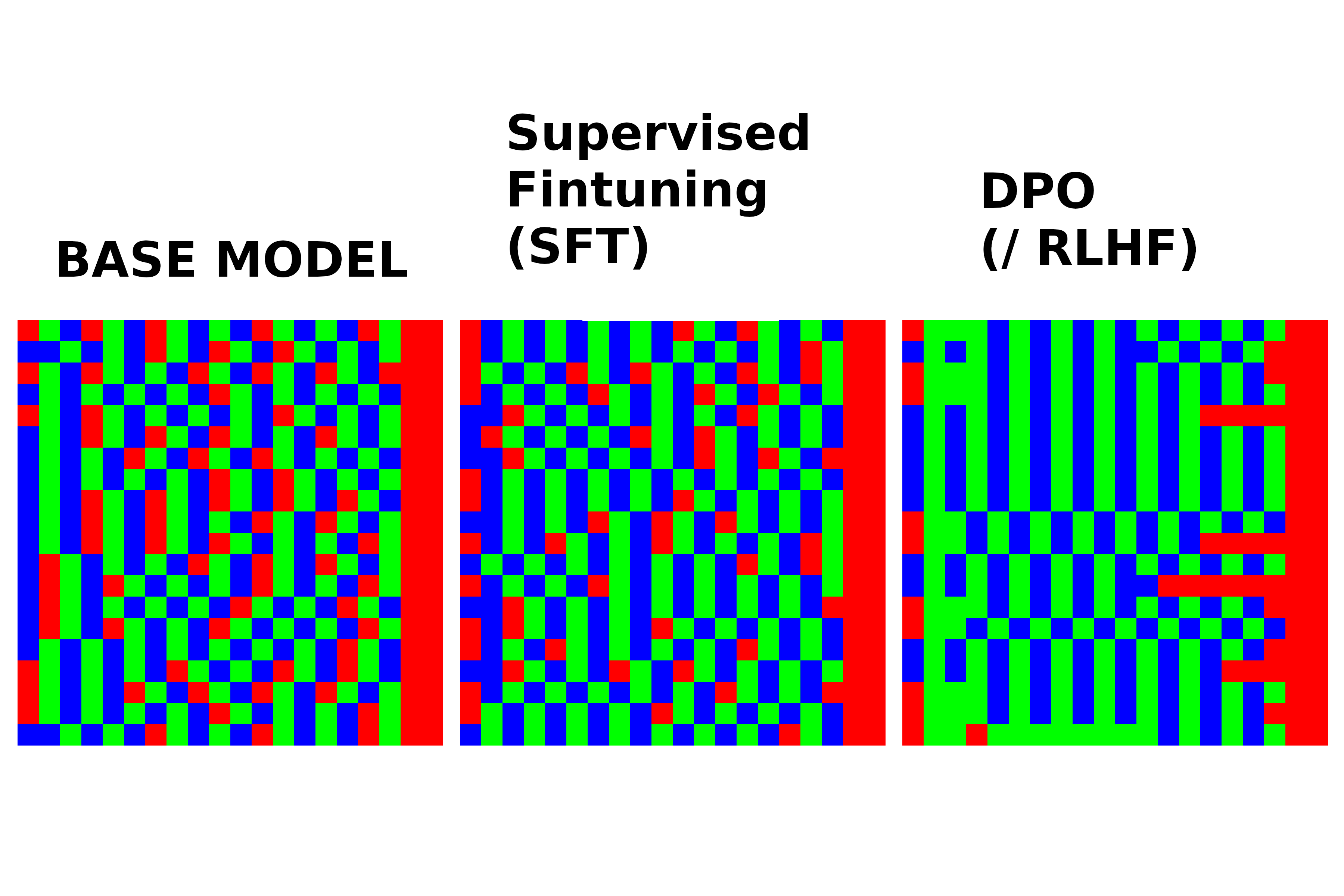
The visual proof is the most compelling part. I generated 20 sequences from each model and plotted them as a 20x20 image, with each tile representing a color.

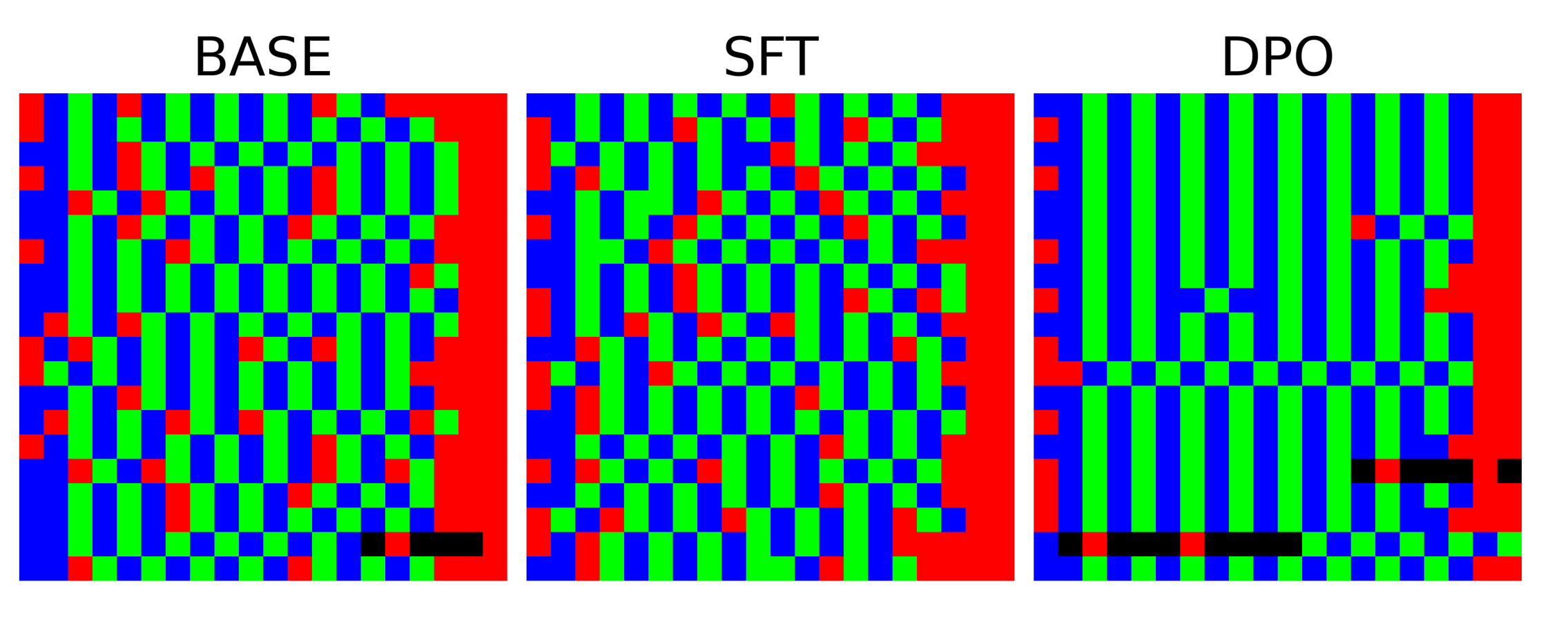
The difference is stark. The BASE and SFT models produce varied, almost random-looking patterns that follow the rules. The DPO model, however, clearly learned a specific strategy: it generates long vertical stripes of …RBGBG…. This rigid, low-entropy pattern is the logical endpoint of the DPO loss function. By rewarding the model for maximizing the probability ratio of ‘chosen’ over ‘rejected’ sequences, the training process effectively forced the model to discover and exploit the single most optimal strategy for gaming the preference score.

What’s the Practical Takeaway?

This simple experiment gives us a powerful mental model for choosing a fine-tuning strategy:

• Use SFT when your goal is imitation. It’s perfect for teaching a model a specific style, format, or knowledge base from a set of high-quality examples. Think “make my chatbot always respond in JSON” or “write in the style of Shakespeare.”
• Use DPO when your goal is optimization. It’s the right choice for teaching a model an abstract preference that is hard to capture in examples alone. Think “make the chatbot funnier,” “be more helpful,” or, in our case, “maximize the occurrence of a specific pattern.”

Why a “Perfect” Dataset Isn’t Enough

In our toy example, we could have generated only the optimal B -> G sequences. But this is precisely where the analogy reveals its most important lesson. In the real world, the preferences we want to teach (like “be more helpful” or “sound more empathetic”) cannot be formalized into a simple, perfect rule. There is no single “perfectly empathetic” response. Human values are complex, subjective, and highly contextual.

This is why alignment techniques like DPO are so powerful. They learn from comparisons (this response is better than that one) to navigate the messy landscape of human preferences where no perfect formula exists.

Ultimately, the best approach depends on your goal. If you want a well-behaved student who can mimic the best, SFT is your tool. If you want a creative problem-solver that can figure out how to win the game, DPO is the way to go.

Basics And Further Reading

• Project Notebook: The complete code and analysis for this experiment is available on GitHub. SFT vs. DPO: A Visual Introduction to LLM Fine-Tuning
• The RLHF Book by Nathan Lambert: An excellent, in-depth resource on Reinforcement Learning from Human Feedback. rlhfbook.com
• Hugging Face Deep RL Course: A hands-on course for learning the fundamentals and applications of Deep Reinforcement Learning. Hugging Face Learn
• Foundations of Deep RL Series by Pieter Abbeel: A comprehensive lecture series on Deep Reinforcement Learning. YouTube Playlist