The Epsilon Trap: When Adam Stops Being Adam

I recently went down a rabbit hole in Andrej Karpathy’s nano-chat repository. While reading through the config files (as one does on a Friday night), a single hyperparameter override caught my eye. It wasn’t a complex architectural change or a new sampling strategy. It was this line:

adamw_kwargs = dict(..., eps=1e-10, ...)

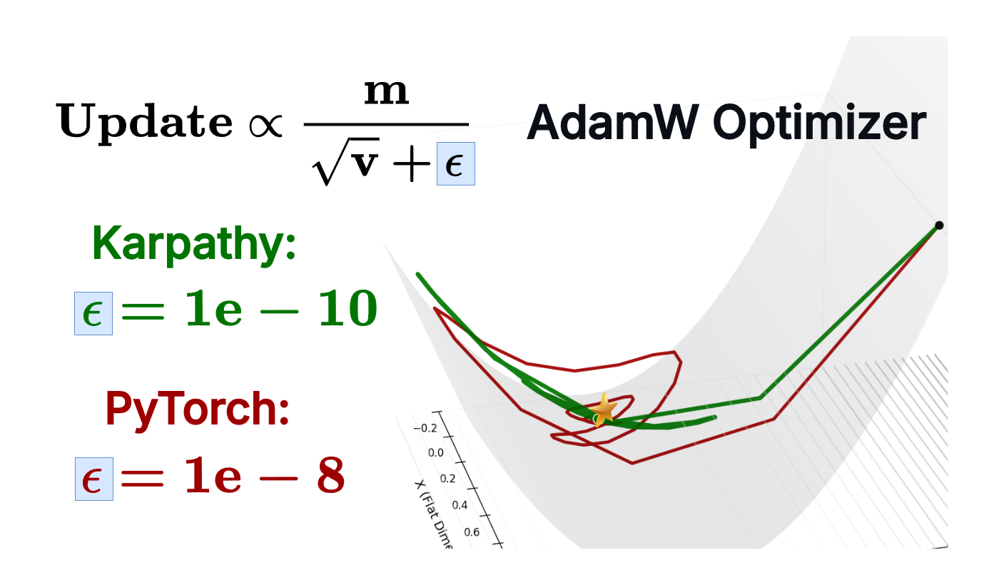
He sets Adam’s epsilon to 1e-10 instead of the PyTorch default of 1e-8.

We usually treat epsilon as a boring “numerical stability” hack : a tiny number added to avoid division by zero. We set it and forget it. But why would Karpathy change it by two orders of magnitude?

It turns out epsilon has a much bigger (:O) story to tell. This parameter actually acts as a threshold that destroys Adam’s scale invariance when your gradients become small.

To understand why, I decided to design a toy experiment to strip down the complexity and see exactly what happens to Adam when it enters the “Epsilon Zone.”

---

The Theory: The Two Faces of Adam

Before running the experiment, let’s build a quick intuition. Mathematically, the Adam update (not AdamW) looks roughly like this:

\[\text{Update} \propto \frac{m}{\sqrt{v} + \epsilon}\]

Note: For simplicity, I’m omitting the bias-correction terms ($1-\beta^t$) to focus on the denominator’s behavior.

Where $m$ is the momentum (Exponentially Weighted Moving Average (EWMA) of past gradients) and $v$ is the variance (EWMA of past squared gradients). There are two distinct regimes of behavior here:

The Adaptive Regime ($\sqrt{v} \gg \epsilon$): This is how Adam is supposed to work. The $\epsilon$ is negligible, and the update becomes:

\[\frac{m}{\sqrt{v}} \approx \frac{g}{|g|} = \text{sign}(g)\]

The magnitude cancels out. This is scale invariance: whether your gradients are huge or tiny, Adam takes steps of roughly the same size.

The SGD Regime ($\sqrt{v} \ll \epsilon$): This is the danger zone. When your gradients drop below a certain threshold, $\epsilon$ dominates the denominator. The update becomes $\frac{m}{\epsilon}$. The denominator is now a constant. Adam loses its adaptivity and the update becomes proportional to the raw momentum term scaled by $\frac{1}{\epsilon}$ effectively behaving like SGD with momentum but with a fixed, potentially inappropriate learning rate.

My hypothesis was simple: The default eps=1e-8 creates a “floor” that acts as a brake on convergence for flat landscapes.

---

The Toy Problem: Racing Down a Micro-Canyon

To test this, I built a “Micro-Canyon” simulation.

I created a 2D loss landscape designed to be ill-conditioned: steep in the Y-axis, but extremely flat in the X-axis.

\[L(x, y) = (x \cdot 10^{-4})^2 + y^2\]

The Micro-Canyon loss landscape: a narrow valley that’s steep in Y but incredibly flat in X. Notice how the contours compress into tight bands along the X-axis; this is where epsilon becomes critical.

This creates a specific challenge:

• The gradient in Y is large (easy to learn).
• The gradient in X is tiny ($\approx 10^{-8}$) (right on the edge of the Pytorch default epsilon).

I ran the optimization with three different “flavors” of epsilon:

• The Stability Hack (1e-6): Often used to prevent NaNs in mixed precision.
• The Default (1e-8): The standard PyTorch setting.
• The Karpathy Choice (1e-10): The value found in nano-chat.

---

The Results: When Epsilon Becomes the Bottleneck

Three Adam optimizers racing to the minimum with different epsilon values. Red (1e-10) takes the optimal path, while blue (1e-6) oscillates chaotically before converging.

The Dark Red Dot (1e-10) behaves like true Adam. It shoots down the steep Y-axis, hits the valley floor, and immediately makes a sharp 90-degree turn. Because $\epsilon$ is smaller than the tiny X-gradients, Adam correctly normalizes the curvature. It skates effortlessly along the flat valley floor to the global minimum with minimal wasted steps.

The Blue Dot (1e-6) converges eventually, but at what cost? It rushes down the Y-axis but then enters a chaotic regime when trying to move in X. Because the X-gradient ($\approx 10^{-8}$) is smaller than epsilon ($10^{-6}$), the adaptive term is dominated by the constant floor. The optimizer loses its sense of direction and begins to oscillate wildly—you can see it spiraling in the left panel and creating a messy trajectory in the right panel. It eventually finds the minimum, but only after wasting hundreds of steps wandering in circles.

The Green Dot (1e-8) sits in the middle. It shows some oscillation but less dramatically than blue. This is the PyTorch default, and while it works, it’s clearly suboptimal compared to the clean, efficient path taken by the 1e-10 configuration.

Mapping the Ceiling

To visualize this transition, we can define the Amplification Factor (or Effective Gain). This measures how much Adam boosts the update relative to the raw gradient, calculated as the ratio between the optimizer’s update size and the product of the learning rate and gradient magnitude:

\[\text{Amplification} = \frac{\text{Update}}{\text{Learning Rate} \times \text{Gradient}}\]

We plot this amplification against the observed gradient magnitudes during optimization (on log scales, with magnitudes decreasing from left to right). The solid lines represent the median trend across binned data points for de-noised visualization, while the faint shaded regions show the interquartile range (IQR) to capture variability in the stochastic updates. Dashed horizontal lines indicate the theoretical maximum amplification ceiling for each epsilon value (approximately $\frac{1}{\epsilon}$).

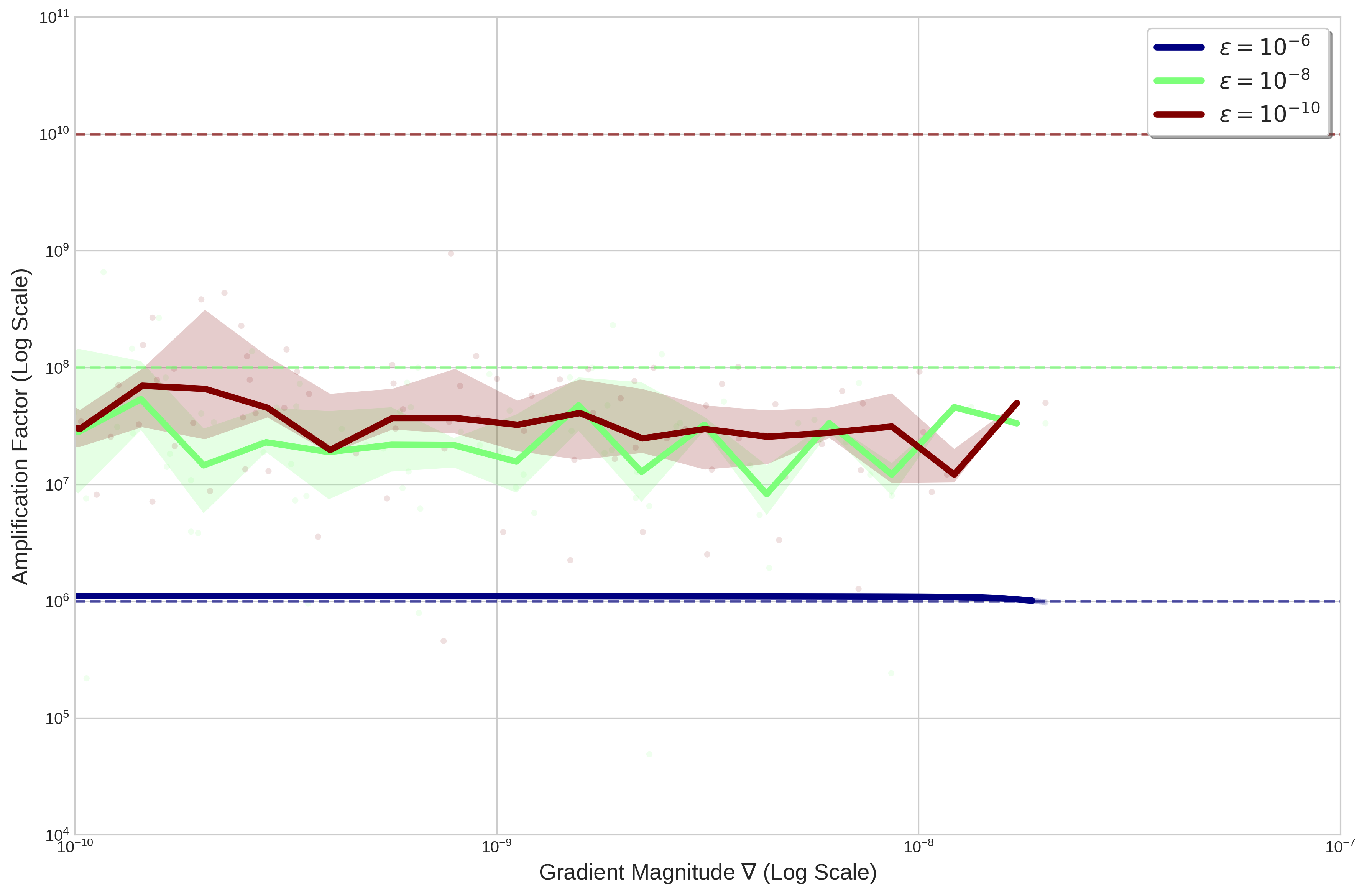The Epsilon Ceiling: Solid lines show the median trend (de-noised) for each configuration. Faint shaded regions show the IQR of the raw stochastic updates. Dashed lines mark the theoretical ceilings.

This plot reveals the “Epsilon Trap” in high resolution:

• The Hard Ceiling (Blue line, $10^{-6}$): The amplification factor is capped at a low level around $10^6$, remaining relatively stable and flat across gradient magnitudes. It shows little to no adaptation as gradients shrink, quickly hitting its limit and behaving more like a non-adaptive optimizer.

• The Middle Ground (Green line, $10^{-8}$): This achieves higher amplification, hovering around $10^8$ with some moderate wiggliness and variation (visible in the IQR shading), indicating partial adaptation before approaching its ceiling.

• The Elevated Plateau (Red line, $10^{-10}$): The amplification reaches the highest levels, up to around $10^9$ in the observed data, but remains relatively flat without a clear increase as gradients get smaller. This allows Adam to maintain stronger boosts in flat regions compared to larger epsilons, though it still encounters practical limits short of its theoretical ceiling (dashed line at $10^{10}$, above the plot’s y-limit).

The “Trust Region” Secret

This isn’t just a quirk of toy problems. I found that this behavior is actually documented in the literature. In his blog post ε, A Nuisance No More, Google Researcher Zack Nado highlights that epsilon acts as a damping term that controls the trust region radius.

• Low Epsilon: “I trust my adaptive curvature estimate, even if the signal is small.”
• High Epsilon: “I don’t trust this tiny signal; I will treat it as noise and fall back to SGD.”

This explains why we see such variance in SOTA configurations, the Karpathy’s nano-chat, but I’ve also found an example on some older models from Google DeepMind like Rainbow DQN,2017 (Deep Q Learning), where they use an eps value of 1.5e-4 for Adam.

Nado also points out a fun inconsistency: PyTorch defaults to 1e-8, while TensorFlow often defaults to 1e-7. It seems even the frameworks can’t agree on where the “floor” should be.

---

Nuance: When Should You Use 1e-8?

So is 1e-10 always better? Clearly not, the default 1e-8 exists for a reason: Float16 Stability. If you are training in pure half-precision (FP16), the smallest normal number is approximately 6e-5, and even accounting for subnormal numbers, the true smallest representable value is around 6e-8. If you set epsilon to 1e-10 in pure FP16 training, it will effectively underflow to zero, causing division-by-zero errors and exploding gradients.

However, most modern LLM training uses BF16 (Bfloat16) or Mixed Precision (FP32 Master Weights). In these cases:

• BF16 has a much wider dynamic range (smallest normal ≈ 1.18e-38), making 1e-10 perfectly safe
• In standard setups (like PyTorch AMP), the optimizer states (momentum and variance) are maintained in FP32 (where 1e-10 is well within range), even if forward/backward passes use FP16.

In both scenarios, 1e-10 is not only safe but often superior to the conservative 1e-8 default.

Code & Data

The complete code for the 3D experiment and animation is available on GitHub.

Citation

If you found this work useful, please cite it as:

Klioui, S. (2026). The Epsilon Trap: When Adam Stops Being Adam. Sifal Klioui Blog. https://sifal.social/posts/The-Epsilon-Trap-When-Adam-Stops-Being-Adam/

Or in BibTeX format:

@article{klioui2026epsilon,
  title   = {The Epsilon Trap: When Adam Stops Being Adam},
  author  = {Klioui, Sifal},
  journal = {Sifal Klioui Blog},
  year    = {2026},
  month   = {Jan},
  url     = {https://sifal.social/posts/The-Epsilon-Trap-When-Adam-Stops-Being-Adam/}
}