The Hidden Beauty of Sinusoidal Positional Encodings in Transformers

A much needed order

Ever wondered how transformers keep track of word order? Let’s dig into one of the most elegant solutions in deep learning: sinusoidal positional encodings. What starts as a simple necessity ends up revealing beautiful mathematical patterns that make these encodings particularly effective.

The Need for Position Information

In traditional sequence models like RNNs, the order of words is implicitly encoded in the sequential processing of the input. However, transformers process all words in parallel to achieve better computational efficiency. This creates a challenge: how do we tell the model that “I park in my sleep” and “I sleep in my park” have different meanings?

This is where positional encodings come in. We need a way to inject position information into our word embeddings without disrupting their learned semantic relationships.

Sinusoidal Positional Encodings

The solution? Add sinusoidal waves of different frequencies to our word embeddings. For each position i and dimension d, we use:

PE(pos, 2i) = sin(pos / 10000^(2i/d_model))
PE(pos, 2i+1) = cos(pos / 10000^(2i/d_model))

At first glance, this might seem arbitrary. Why sines and cosines? Why these specific frequencies? Let’s visualize what happens when we compute the dot products between different positions.

Visualizing the Pattern

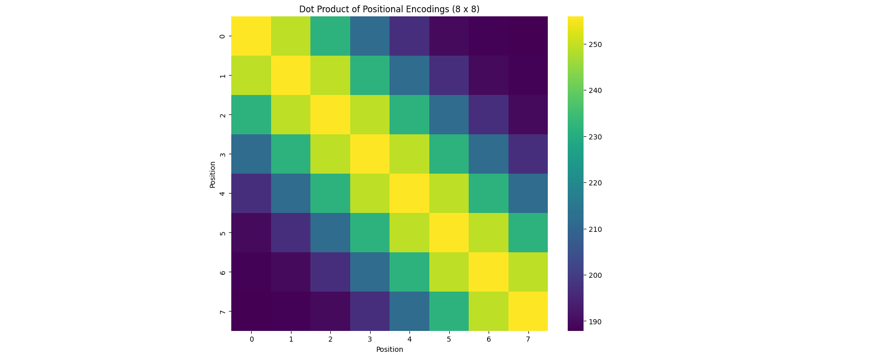
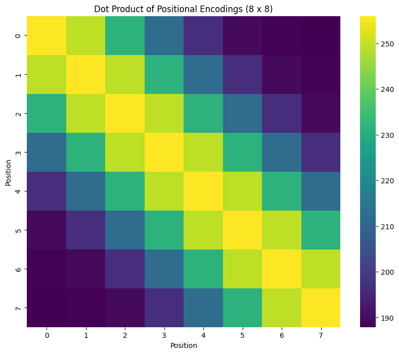
When we plot the dot products between positional encodings as a heatmap, something interesting emerges. Here’s what we get when we look at the first 8 positions:

# Initialize positional encoding
d_model = 512
max_len = 8
pos_enc = PositionalEncoding(d_model, max_len=max_len)

# Extract encodings and compute dot products
pe = pos_enc.pe.squeeze(0)[:max_len]
dot_product_matrix = torch.matmul(pe, pe.T)

We notice something striking: the values along each diagonal seem to be identical. This isn’t a coincidence – it’s a fundamental property of these encodings!

Toeplitz matrices

What we’re looking at is called a Toeplitz matrix – A Toeplitz matrix is a matrix where each descending diagonal from left to right is constant, meaning \(D_{ij} = D_{i+1, j+1}\) for all \(i, j\), or more formally, \(D_{ij} = D_{i-k, j-k}\) for any integer \(k\).

Let’s break down why the dot product matrix of sinusoidal positional encodings has this property and explore its implications.

Mathematical Proof of the Toeplitz Structure

Given the sinusoidal positional encoding at position \(i\) as:

\[\begin{equation} \text{PE}(i) = \left( \sin(i \cdot \omega_1), \cos(i \cdot \omega_1), \sin(i \cdot \omega_2), \cos(i \cdot \omega_2), \ldots \right) \end{equation}\]

where \(\omega_n = \frac{1}{10000^{2n / d_{\text{model}}}}\) for each frequency \(n\).

Now, the dot product between the positional encodings at two positions \(i\) and \(j\) is:

\[\begin{equation} D_{ij} = \text{PE}(i) \cdot \text{PE}(j) = \sum_{k=1}^{d_{\text{model}}/2} \left( \sin(i \cdot \omega_k) \sin(j \cdot \omega_k) + \cos(i \cdot \omega_k) \cos(j \cdot \omega_k) \right) \end{equation}\]

Using the trigonometric identity \(\sin(x)\sin(y) + \cos(x)\cos(y) = \cos(x - y)\), we can rewrite this as:

\[\begin{equation} D_{ij} = \sum_{k=1}^{d_{\text{model}}/2} \cos((i - j) \cdot \omega_k) \end{equation}\]

Thus, \(D_{ij}\) depends only on the difference \(i - j\), not on the specific values of \(i\) and \(j\). This dependency on \(i - j\) alone means that the matrix \(D\) is indeed Toeplitz.

Implications of the Toeplitz Structure

1. Shift-Invariance: A Toeplitz matrix implies that the relationship between positional encodings is shift-invariant. This means that the similarity (dot product) between positional encodings only depends on how far apart the positions are, not on their absolute values. For example, the similarity between positions 1 and 2 will be the same as between positions 80 and 81.

2. Translation of Positional Differences: Since the entries depend only on positional differences, the Toeplitz structure in the positional encoding matrix reflects that the transformer can focus on relative positions rather than absolute positions, aligning with its role in capturing relationships between words regardless of their specific positions in a sentence.

Let’s check this property with some concrete examples:

# Get positional encodings for positions 1, 2, 80, and 81
pe = pos_enc.pe.squeeze(0)  # Remove batch dimension to get (max_len, d_model)
pos_1 = pe[1]               # Positional encoding at position 1
pos_2 = pe[2]               # Positional encoding at position 2
pos_80 = pe[80]             # Positional encoding at position 80
pos_81 = pe[81]             # Positional encoding at position 81

# Calculate dot products
dot_1_2 = torch.dot(pos_1, pos_2).item()
dot_2_1 = torch.dot(pos_2, pos_1).item()
dot_80_81 = torch.dot(pos_80, pos_81).item()
dot_1_80 = torch.dot(pos_1, pos_80).item()
dot_2_81 = torch.dot(pos_2, pos_81).item()

print(f"Dot product between position 1 and 2: {dot_1_2}")
print(f"Dot product between position 2 and 1: {dot_2_1}")
print('\n')
print(f"Dot product between position 80 and 81: {dot_80_81}")
print('\n')
print(f"Dot product between position 1 and 80: {dot_1_80}")
print(f"Dot product between position 2 and 81: {dot_2_81}")

Dot product between position 1 and 2: 249.10211181640625
Dot product between position 2 and 1: 249.10211181640625

Dot product between position 80 and 81: 249.1020965576172

Dot product between position 1 and 80: 117.52901458740234
Dot product between position 2 and 81: 117.52900695800781

Conclusion

What started as a practical need to encode position information led us to discover a mathematically elegant solution with beautiful properties. The sinusoidal positional encoding isn’t just a hack – it’s a carefully designed component that brings together trigonometry, linear algebra, and deep learning in a surprisingly harmonious way.

Next time you’re working with transformers, remember that even in their smallest components, there might be hidden mathematical beauty waiting to be discovered!

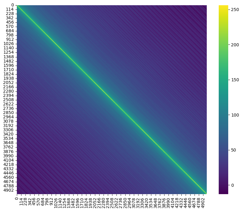
Just for the fun here’s a bigger one!