Towards a Bitter Lesson of Optimization: When Neural Networks Write Their Own Update Rules
We explore what can be the future of neural network parameter optimization
We work in an industry defined by Richard Sutton’s famous “Bitter Lesson”. The lesson dictates that hand-crafted, human-designed features (like SIFT or HOG in computer vision) are ultimately always beaten by general methods that leverage computation and learning.
When we look at the gradients flowing through a neural network during training, they aren’t just pure noise. The distribution of these gradients follows specific, exploitable structural patterns over time. Yet, ironically, the very algorithms we use to train these networks, like Adam, are entirely hand-designed by humans. We rely on analytical insights, manual heuristics, and rigid mathematical formulas to navigate unimaginably complex loss landscapes.
It turns out, DeepMind had this exact same realization back in 2016 in their seminal paper: Learning to learn by gradient descent by gradient descent. They asked a simple question: What if we cast the design of the optimization algorithm itself as a learning problem?
Let’s strip down the math and build an intuition for what happens when we let an AI optimize another AI.
Motivation: Limits of Hand-Crafted Optimizers
Before we replace Adam, we have to understand the fundamental ceiling it hits: The No Free Lunch (NFL) Theorem for Optimization.
The NFL theorem mathematically proves that across all possible optimization problems, no algorithm is universally optimal. Adam works well because it implicitly assumes a specific distribution of gradients, using exponentially weighted moving averages of past gradients to smooth out noise and adaptively scale step sizes. It is imbued with human-engineered structural biases tailored specifically for the continuous loss landscapes we typically encounter.
But just as Computer Vision moved from hand-crafted structural biases to learning them directly from data (like CNNs learning spatial hierarchies or Vision Transformers learning patch interactions), shouldn’t we do the same for optimization? If human researchers can design Adam by making assumptions about deep learning landscapes, a neural network should be able to integrate (or better yet, learn) the perfect, highly-specialized inductive biases just by observing the distribution of gradients directly.
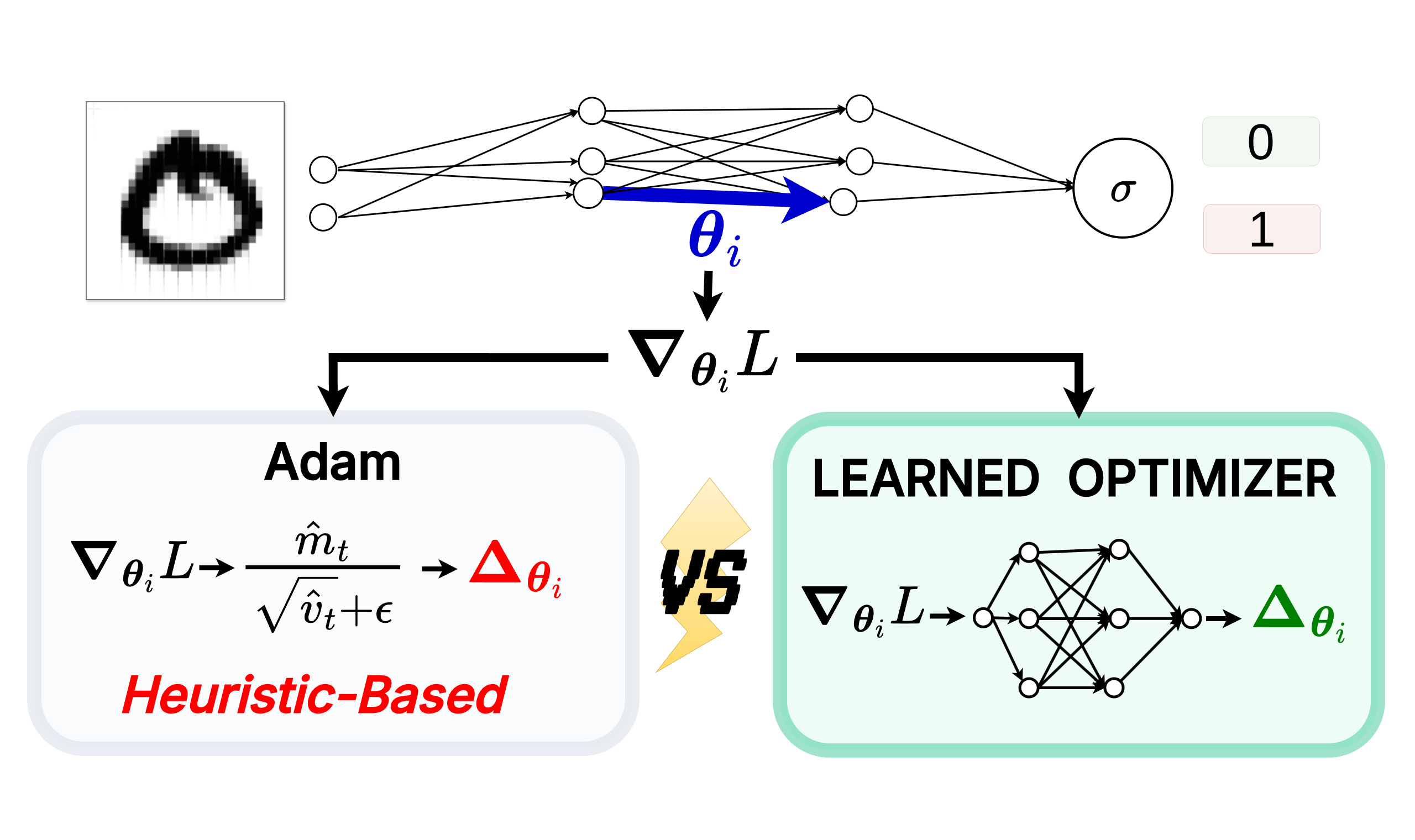
Theory: Optimizer vs Optimizee
To do this, we need to set up a two-loop system. We have:
- The Optimizee (\(f\)): The base model we are actually trying to train (e.g., a simple image classifier). Its parameters are \(\theta\).
- The Optimizer (\(g\)): A neural network parameterized by \(\phi\). Its job is to ingest a feature vector, primarily the optimizee’s gradient, possibly other features like running moments potentially at different decaying regimes, and output the parameter update for \(\theta\).
Mathematically, a standard gradient descent update looks like this: \(\theta_{t+1} = \theta_t - \alpha \nabla f(\theta_t)\)
In our meta-learning setup, we replace the hand-crafted learning rate (\(\alpha\)) and the rigid gradient step with the output of our parameterized optimizer:
\[\theta_{t+1} = \theta_t + \underbrace{g_t(\nabla f(\theta_t), \phi)}_{\Delta \theta_i^t}\]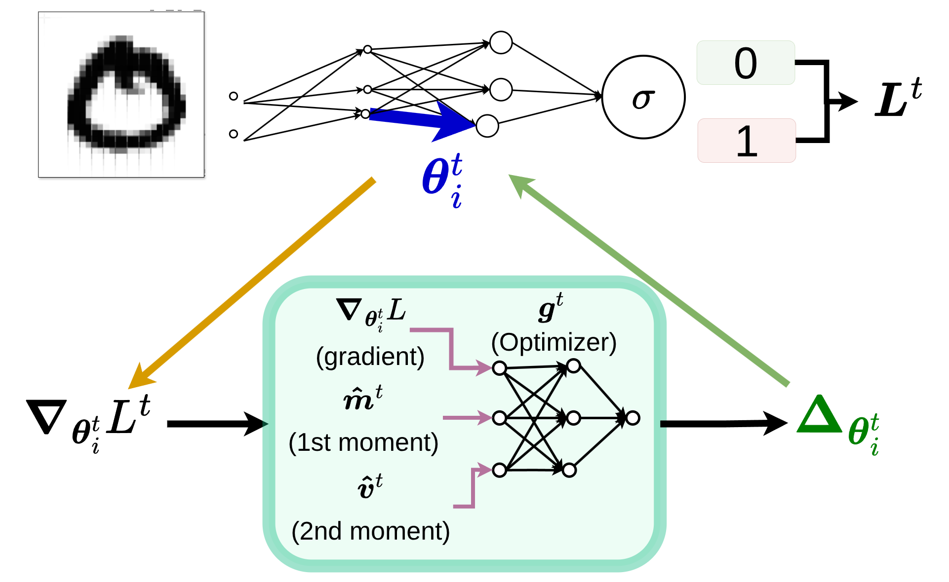 The inference phase: the optimizee’s loss gradients flow into the optimizer, which predicts the parameter step \(\Delta \theta_i^t\) to apply back to the optimizee.
Two Objectives
Crucially, we must distinguish between the objectives of these two networks. They are playing two different games.
The optimizee is trying to minimize its standard task loss, \(f(\theta)\), to get better at classifying images or generating text.
The optimizer, however, has its own unique loss function, \(\mathcal{L}(\phi)\). Its goal is to minimize the expected sum of the optimizee’s losses across an entire trajectory of training steps \(T\):
\[\mathcal{L}(\phi) = \mathbb{E}_f \left[ \sum_{t=1}^T w_t f(\theta_t) \right]\]where \(w_t\) are arbitrary weights assigned to each timestep. In their experiments, Andrychowicz et al. opt to use \(w_t = 1\) for all \(t\). The meta-optimizer is trained to produce update steps that minimize the optimizee loss across the whole trajectory.
Trajectory Loss
Why sum over the entire trajectory instead of just evaluating the final loss at step \(T\)? If only the final step is weighted, meaning if you use:
\[w_t = \mathbf{1}[t = T]\]then only the final step contributes. This leads to a poor gradient signal during training because earlier steps do not get supervision. By weighting every step, we force the optimizer to care about the dynamics. It is penalized for slow convergence and rewarded for descending quickly, smoothly, and stably.
For those familiar with Reinforcement Learning, assigning weights to intermediate steps in a trajectory strongly resembles the discount factor (\(\gamma\)) used to compute the return.
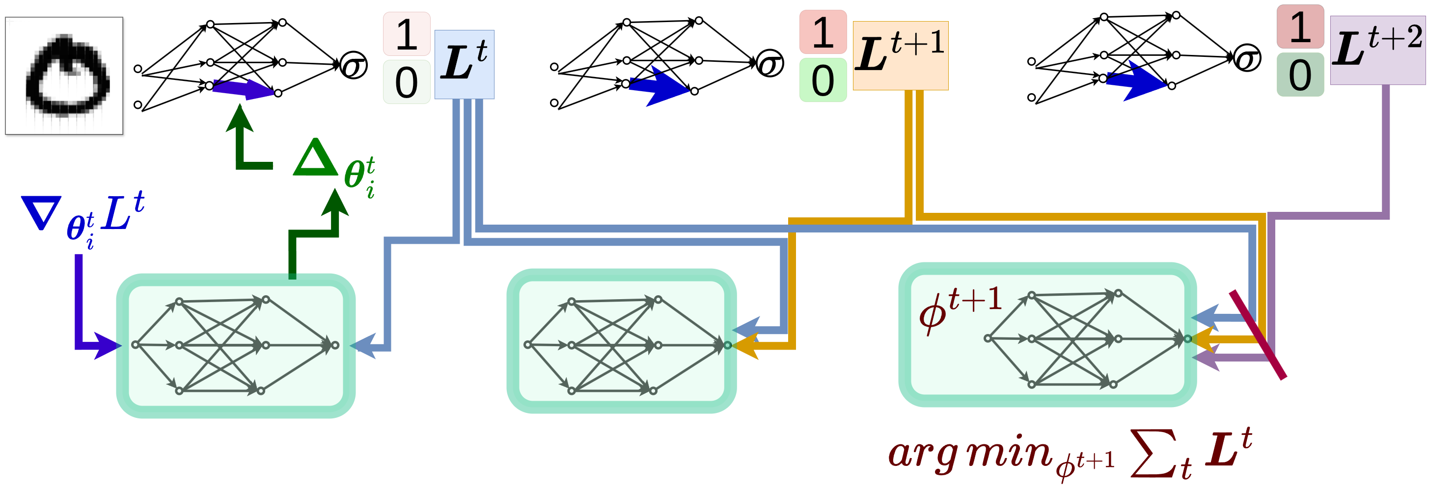 The training phase: the optimizer (green blocks) is trained by backpropagating through the unrolled steps to minimize the trajectory loss over time.
Meta-Generalization
Let’s look back at our objective function: \(\mathcal{L}(\phi) = \mathbb{E}_f \left[ \sum_{t=1}^T w_t f(\theta_t) \right]\). Notice the expectation operator \(\mathbb{E}_f\) at the front. The optimizer isn’t just trying to minimize the trajectory loss for a single neural network on a single dataset. It is optimizing over a distribution of functions.
Because the optimizer is trained over a distribution of tasks, it learns the statistical regularities of that specific distribution. It is not learning a mathematically universal optimizer. Rather, it is learning an amortized optimizer that is heavily specialized to the distribution of tasks it saw during meta-training.
The true goal here is meta-generalization. We want the optimizer to learn update rules that generalize across different architectures, tasks, hidden sizes, and number of layers. For example, an optimizer trained on a 2-hidden-layer network with a specific hidden size classifying MNIST digits should ideally be able to seamlessly drop in and optimize a 3-hidden-layer network with a different hidden capacity classifying dogs vs. cats. It’s learning the underlying physics of gradient descent, not just memorizing the fastest route down a single, specific hill.
 Meta-Generalization: The central optimizer learns to optimize across a distribution of different architectures, tasks, hidden sizes, and number of layers.
However, there is a catch. Empirically, it has been shown that while these optimizers can generalize across architectures and datasets, they often fail to generalize across fundamentally different activation functions. For instance, an optimizer trained on networks using Sigmoid activations does not generalize to networks using ReLU activations (though, to be fair, they primarily tested only between these two). The distinct geometry created by different activation functions alters the loss landscape so drastically that the learned inductive biases no longer apply.
This failure is expected because different network architectures induce completely different loss landscape geometries. The learned update rule is intrinsically dependent on those specific geometries. Therefore, generalization across fundamentally different settings is inherently limited by the underlying task distribution.
Training: Stability vs Bias
The Hessian
When we actually try to minimize this trajectory loss \(\mathcal{L}(\phi)\) by backpropagating through the optimization steps, the math gets gnarly. Let’s see exactly where this complexity comes from by starting from our parameter update rule.
For simplicity, and without a loss of generalization, let’s assume our optimizer \(g\) takes in only the previous gradient \(\nabla_{t-1}\) and its weights \(\phi\):
\[\theta_t = \theta_{t-1} + g(\nabla_{t-1}, \phi)\]To train the optimizer, we need to know how a change in its weights \(\phi\) affects the optimizee’s parameters \(\theta_t\). So, we take the partial derivative of both sides with respect to \(\phi\). By applying the multi-variable chain rule to \(g\), we get:
\[\frac{\partial \theta_t}{\partial \phi} = \frac{\partial \theta_{t-1}}{\partial \phi} + \frac{\partial g}{\partial \phi} + \frac{\partial g}{\partial \nabla_{t-1}} \cdot \frac{\partial \nabla_{t-1}}{\partial \phi}\]Take a close look at the gradient term in that expansion: \(\frac{\partial \nabla_{t-1}}{\partial \phi}\). How does the previous gradient change with respect to the optimizer’s weights? By applying the chain rule once more, we reveal the core mathematical challenge:
\[\frac{\partial \nabla_{t-1}}{\partial \phi} = \frac{\partial \nabla_{t-1}}{\partial \theta_{t-1}} \cdot \frac{\partial \theta_{t-1}}{\partial \phi}\]Notice that first term on the right side: \(\frac{\partial \nabla_{t-1}}{\partial \theta_{t-1}}\). Since \(\nabla_{t-1}\) is already the first derivative of the loss function \(f\), taking its derivative with respect to \(\theta_{t-1}\) gives you the second derivative of the loss function. That is the Hessian!
Computing this matrix at every step is prohibitively expensive. Implementations like Andrychowicz’s explicitly chose to ignore these second-order derivatives to save resources, essentially assuming the gradients of the optimizee don’t depend on the optimizer’s parameters (setting \(\frac{\partial \nabla_{t-1}}{\partial \phi} \approx 0\)).
Truncation
Furthermore, when you unwrap the derivative of the parameters over the time trajectory to train the optimizer, you get the unrolled learned optimizer gradient:
\[\frac{d\theta_t}{d\phi} = \sum_{k=0}^{t-1} \left( \prod_{j=k+1}^{t-1} \frac{\partial \theta_{j+1}}{\partial \theta_j} \right) \frac{\partial g_k}{\partial \phi}\]Show Proof
You are essentially computing the sum of the products of the Jacobians. The product of Jacobians \(\prod_{j=k+1}^{t-1} \frac{\partial \theta_{j+1}}{\partial \theta_j}\) grows exponentially with the number of terms if any of these Jacobians has a spectral radius (maximum eigenvalue) greater than 1. (For those who want to explore the math a a bit more, here are some keywords :)) : dynamical systems, positive maximum Lyapunov exponent). This means that, on average over many steps, the cumulative product of the Jacobians causes trajectories to diverge exponentially (even if individual Jacobians occasionally contract). Just like in standard Recurrent Neural Networks (RNNs), multiplying many Jacobians together across a long sequence tends to cause gradients to explode or vanish.
This process is mathematically equivalent to multiplying many matrices together over time. The norm of this product behaves exponentially: it grows uncontrollably if the spectral radius is greater than 1, and shrinks to zero if it is less than 1. This is the exact same fundamental instability that plagues the training of standard Recurrent Neural Networks (RNNs).
Because of this, we cannot empirically sum over the entire training trajectory \(T\). To fix this, we apply truncation. For those familiar with training RNNs, this is akin to Truncated Backpropagation Through Time (TBPTT). We only unroll the optimizer for a fixed, shorter window of steps before updating its weights. This presents a major practical advantage: rather than waiting hours or days for a full training trajectory to complete just to extract a single meta-gradient, truncation allows us to make rapid, frequent updates to the optimizer’s parameters.
Crucially, truncation does not simply approximate the original objective. It fundamentally changes the objective. The original objective was to optimize performance over the full trajectory. The truncated objective is to optimize performance over a short, isolated window.
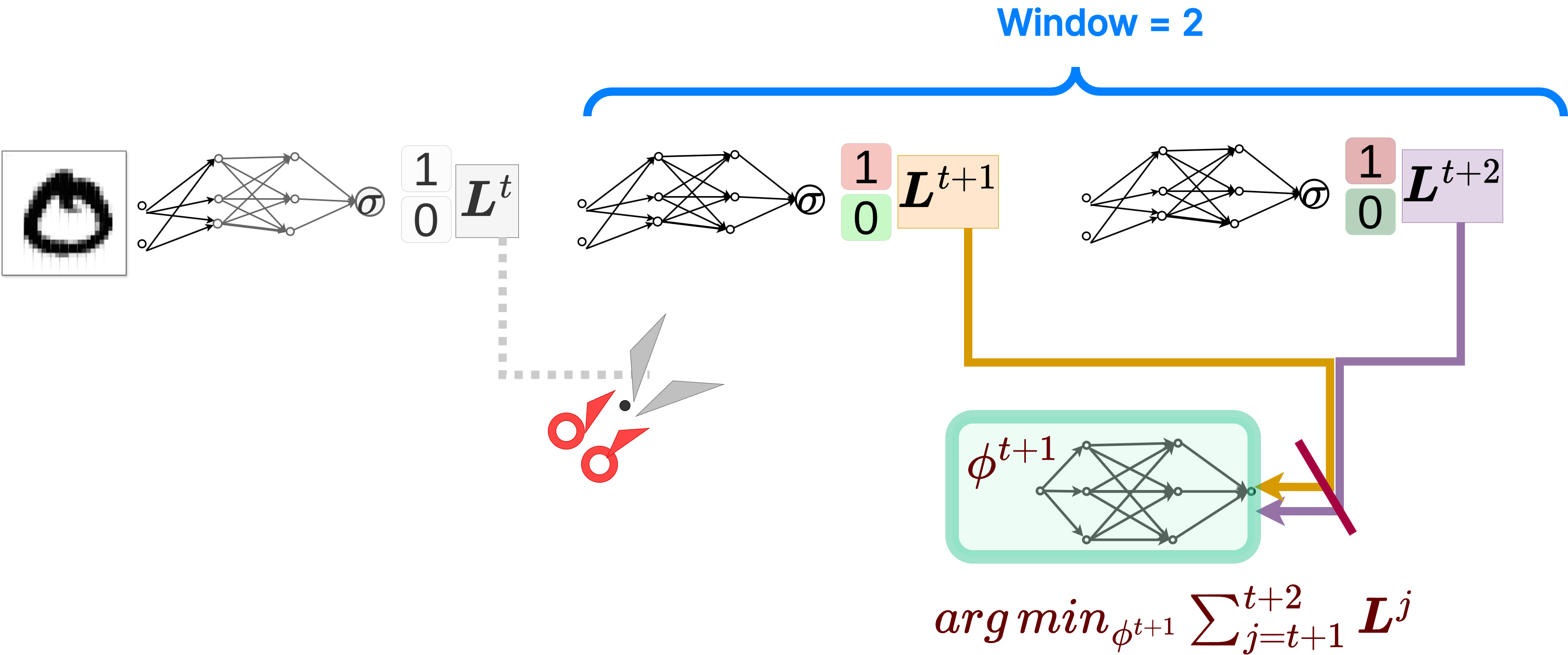 Truncated loss computation, showing an example with a window of 2 steps.
While truncation saves us from exploding gradients and memory exhaustion—and critically enables these highly frequent updates—it introduces a new problem: it causes biased updates. This bias is highly systematic. It heavily favors short-term improvements. Because the optimizer cannot see beyond the truncation window, it is no longer learning long-term convergence behavior. It is strictly learning a short-horizon strategy. The optimizer becomes inherently blind to the long-term consequences of its steps beyond the truncation window, optimizing for short-term gains at the potential expense of long-term convergence.
Optimization Granularity
Now that we know how the optimizer is trained, how do we actually wire it up? This meta-optimization can be implemented at different levels of granularity: exclusively at the parameter level (coordinate-wise), inclusively at the tensor level, or even globally at the neural network level. Each approach comes with significant trade-offs in memory, compute, expressivity, and generalizability.
Before we look at the specific architectures, we must formalize the sheer computational cost. Let \(N\) be the total number of parameters in the optimizee and \(B\) be the batch size. The total cost of a single training step, \(C_{step}\), is the sum of the standard forward and backward pass, \(C_{grad}(B, N)\), and the cost of executing the parameter update, \(C_{opt}(N)\):
\[C_{step} = C_{grad}(B, N) + C_{opt}(N)\]The cost of the gradients scales as \(\mathcal{O}(B \cdot N)\). A key insight here is regarding the relative compute overhead \(\rho = C_{opt} / C_{grad}\). Since \(C_{grad}\) scales with the batch size \(B\) but \(C_{opt}\) is completely independent of \(B\), we encounter what is known as the Theorem of Optimizer Dilution. The relative computational overhead of the learned optimizer essentially vanishes as your batch size grows:
\[\lim_{B \to \infty} \rho = \lim_{B \to \infty} \frac{C_{opt}(N)}{\mathcal{O}(B \cdot N)} = 0\]Free Compute in the Distributed Regime? When scaling Data Parallelism to thousands of GPUs, throughput efficiency eventually drops. The communication overhead (specifically reduction operations and ring latency) grows to a point where it can no longer be overlapped with computation, leaving GPUs idling. As highlighted in the Hugging Face Ultrascale Playbook, communication becomes the ultimate bottleneck. Since we are already bottlenecked by network transfers, we effectively have “free” compute cycles. I am really curious if this overlapping capacity could actually be beneficial in practice. Could we theoretically inflate the computation step by running a heavier learned optimizer? If carefully pipelined, perhaps this extra meta-optimization compute could be hidden behind the network latency, giving us smarter parameter updates for zero extra wall-clock time! I don’t know for sure, but it is an exciting possibility to think about.
However, the raw cost of \(C_{opt}\) and the memory overhead depend entirely on the level of granularity we choose. Let’s break down the complexities of each approach.
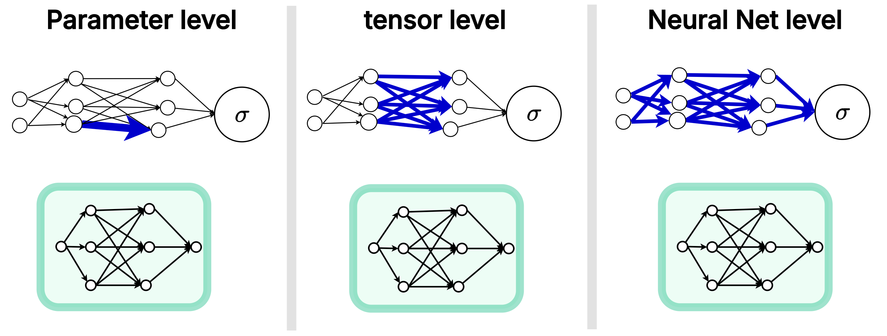 Different levels of meta-optimization. Crucially, in approaches like the parameter level, the optimizer instance is shared across all parameters.
Parameter-Level Optimization
If our optimizer had full, unconstrained access to the global loss landscape, mapping an \(N\)-dimensional gradient vector to an \(N\)-dimensional update vector, the compute would scale as \(\mathcal{O}(N^2)\). For a modern 1 billion parameter model, that is \(10^{18}\) operations per step. This is physically impossible.
To make learned optimizers practical, we typically choose the parameter level. We do not build a separate optimizer network for every single parameter. That would be astronomically massive. Instead, we share the same optimizer’s neural network weights (\(\phi\)) across all parameters (as seen in the left panel above), maintaining a separate, independent hidden state for each.
Because the exact same optimizer is applied independently to each parameter, the update rule takes the form \(\Delta \theta_i = g(\nabla_i, \text{features}_i; \phi)\). In this setup, the optimizer only sees local information. It cannot natively model interactions or correlations between different parameters.
If \(\left\| \phi \right\|_{\text{opt}}\) is the number of weights in this learned optimizer (often instantiated as a simple MLP, though any lightweight architecture could be used), the compute cost drops drastically to \(C_{opt} = \mathcal{O}(N \cdot \left\| \phi \right\|_{\text{opt}})\). While linear, the compute tax is still exceptionally high because the optimizer must execute its forward pass \(N\) times per step (once for every single parameter).
To keep memory and compute tractable, we are forced to keep \(\left\| \phi \right\|_{\text{opt}}\) extremely small. However, this is not necessarily a bad thing. For instance, Metz et al. (2022) designed an optimizer called small_fc_lopt, using an ultra-tiny MLP with only 197 parameters as their architecture of choice. Despite its minuscule size, it is incredibly rich in context. Instead of just passing the raw gradient, this optimizer processes 39 distinct input features per coordinate. These include local states (parameter values, gradients, and multiple momentum accumulators), scale-invariant quantities (like AdaFactor-normalized statistics), and global training context (time features that give the optimizer phase awareness, letting it know if it is early or late in training).
This architectural choice forces the optimizer into the restricted class of coordinate-wise methods. It makes the learned optimizer equivalent in underlying structure to algorithms like SGD, Adam, and RMSProp.
By restricting the optimizer to a shared, parameter-level architecture, it fundamentally behaves like Adam (tracking 1st and 2nd moments independently per parameter) but supercharged. It learns to optimally combine multi-timescale signals and momentum variations without the catastrophic memory overhead of a larger global network.
However, we must recognize the structural ceiling here. Even if entirely learned, the optimizer is still just a diagonal preconditioner. It cannot represent full loss curvature because there is absolutely no cross-parameter coupling. Therefore, this paradigm is fundamentally just a highly parameterized refinement of Adam-like methods, not a true departure from them.
Tensor- and Network-Level Optimization
What if we want more expressivity? In “Practical Tradeoffs Between Memory, Compute And Performance In Learned Optimizers” (Metz et al., 2022), researchers analyzed hierarchical optimizers that operate at the parameter, tensor, and global levels simultaneously.
The results showed that while hierarchical approaches distribute the heavy computation across shared levels (leading to sub-linear runtime scaling per parameter), the absolute compute and memory costs remain massive. The compute complexity becomes \(\mathcal{O}(N \cdot \left\| \phi \right\|_{\text{param}} + \text{Tensors} \cdot \left\| \phi \right\|_{\text{hierarchical}})\), where \(\phi_{\text{param}}\) and \(\phi_{\text{hierarchical}}\) represent the capacities of the parameter-level and higher-level networks (frequently instantiated in literature as MLPs and RNNs, respectively, though the framework applies to any architecture). The memory footprint also balloons because the system must store global states, per-tensor states, and per-parameter states all at once.
It is interesting to see that the idea of using tensor-level and neural-network-level optimization was present and studied at that time. The practical limitations of isolated scalars led researchers to explore hierarchical optimizers to treat entire weight matrices holistically. This early shift paved the theoretical groundwork for the highly efficient, matrix-focused optimizers making waves today, like Muon.
Layer-Wise Optimization
This concept of isolated optimization also extends elegantly to the layer level.
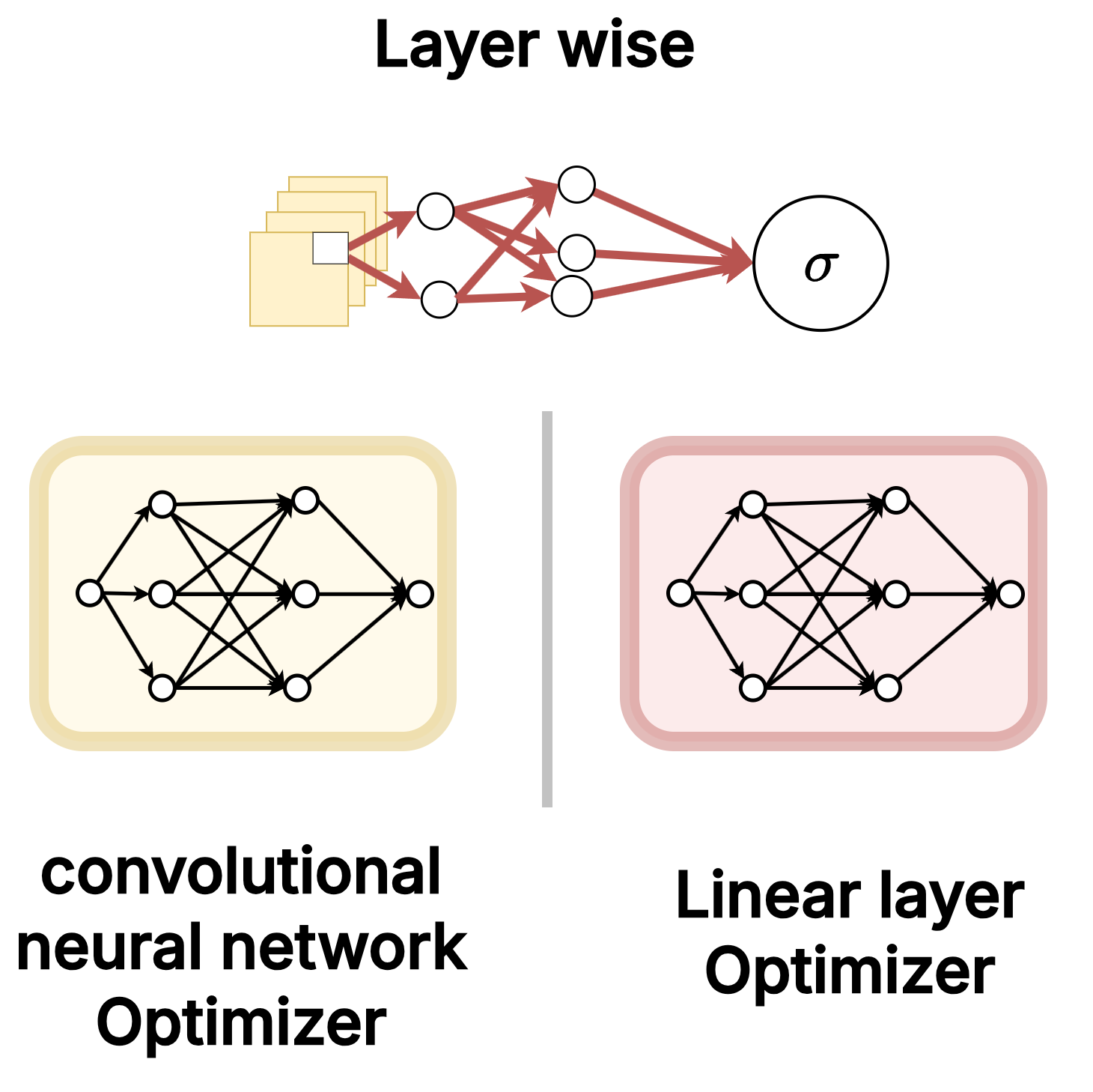 Assigning different learned optimizer instances to different neural network layer architectures.
Complexity-wise, layer-wise optimization shares the exact same linear \(\mathcal{O}(N \cdot \left\| \phi \right\|_{\text{opt}})\) cost as the parameter level. However, it partitions the parameters so that distinct optimizer instances handle distinct architectures.
And this isn’t just about being creative or fancy. The gradient dynamics of linear layers and convolutional layers are fundamentally different. As the DeepMind paper demonstrated, it is empirically highly beneficial to use different optimizer instances tailored to specific architectures. By assigning one learned optimizer exclusively to updating convolutional layers, and an entirely different one tailored for fully-connected linear layers, each optimizer instance is able to learn and exploit the highly specific update dynamics required for that particular architecture without incurring any additional asymptotic compute cost.
Scaling Limits
Long-Horizon Credit Assignment
As we established, gradients depend on long chains of Jacobians. This directly leads to severe mathematical instability. To counter this, we apply truncation, which fundamentally changes the objective. As a result, the optimizer stops learning how to converge over a full training run and instead learns a short-term, greedy behavior.
Expressivity vs Scalability
A fully expressive optimizer would require \(\mathcal{O}(N^2)\) compute to map gradients to updates globally. To make this tractable, we rely on parameter-level sharing. This restricts us entirely to coordinate-wise updates. The result is severely limited expressivity, with no true second-order structure or cross-parameter awareness.
Distribution Dependence
The optimizer is trained over an expectation \(\mathbb{E}_f\). It learns heavily distribution-specific behavior to minimize that expected loss. When the task distribution shifts in geometry or scale, the learned inductive biases fail.
The limitation here is not just a computational difficulty. It is a fundamental mismatch between the true objective (optimizing full, complex trajectories) and what we can realistically optimize (short, local, disconnected signals).
Practical Implementations
PyTorch Based
On a practical note, it is encouraging to see tooling starting to emerge around this paradigm. PyLO is a PyTorch library that provides drop-in replacements for standard optimizers with learned alternatives, complete with CUDA-accelerated kernels. What I find particularly exciting is their Hugging Face Hub integration: meta-trained optimizers can be pushed and pulled from the Hub just like model weights. This resonates with something I had been imagining independently - a future where models don’t just ship their weights, but also bundle the learned optimizer they were trained with. If a model was meta-trained alongside a specific optimizer tuned to its gradient geometry, fine-tuning on a downstream task with that same optimizer could be significantly more efficient than defaulting back to Adam.
To see just how seamless this transition is, we can look at the PyLO examples repository. Swapping Adam for a learned optimizer like VeLO is quite literally a one-line code change:
1
2
3
4
5
6
7
8
9
10
11
12
13
14
15
import torch
from pylo.optim import VeLO_CUDA

# Initialize a model
model = torch.nn.Linear(10, 2)

# Create a learned optimizer instance
optimizer = VeLO_CUDA(model.parameters())

# Use it like any PyTorch optimizer
for epoch in range(10):
    optimizer.zero_grad()
    loss = loss_fn(model(input), target)
    loss.backward()
    optimizer.step(loss) # pass the loss
JAX Based
For those working in the JAX ecosystem, there is also the learned_optimization library by Google (Metz et al., 2022). From skimming through the codebase, it seems to offer more flexibility for custom meta-training and intricate architectures. However, I did struggle to make it run locally. It seems to not really be maintained anymore, leading to a tangle of dependency issues. If you want to experiment with it, I put together a notebook that fixes the dependency conflicts and gets the library running.
To see this in action, I used the notebook to meta-train a toy learned optimizer from scratch. The setup is straightforward: a simple binary classification inner task, a coordinate-wise MLP acting as the optimizer, and explicit Truncated Backpropagation Through Time (TBPTT) with a window of 10 steps to compute the meta-gradients.
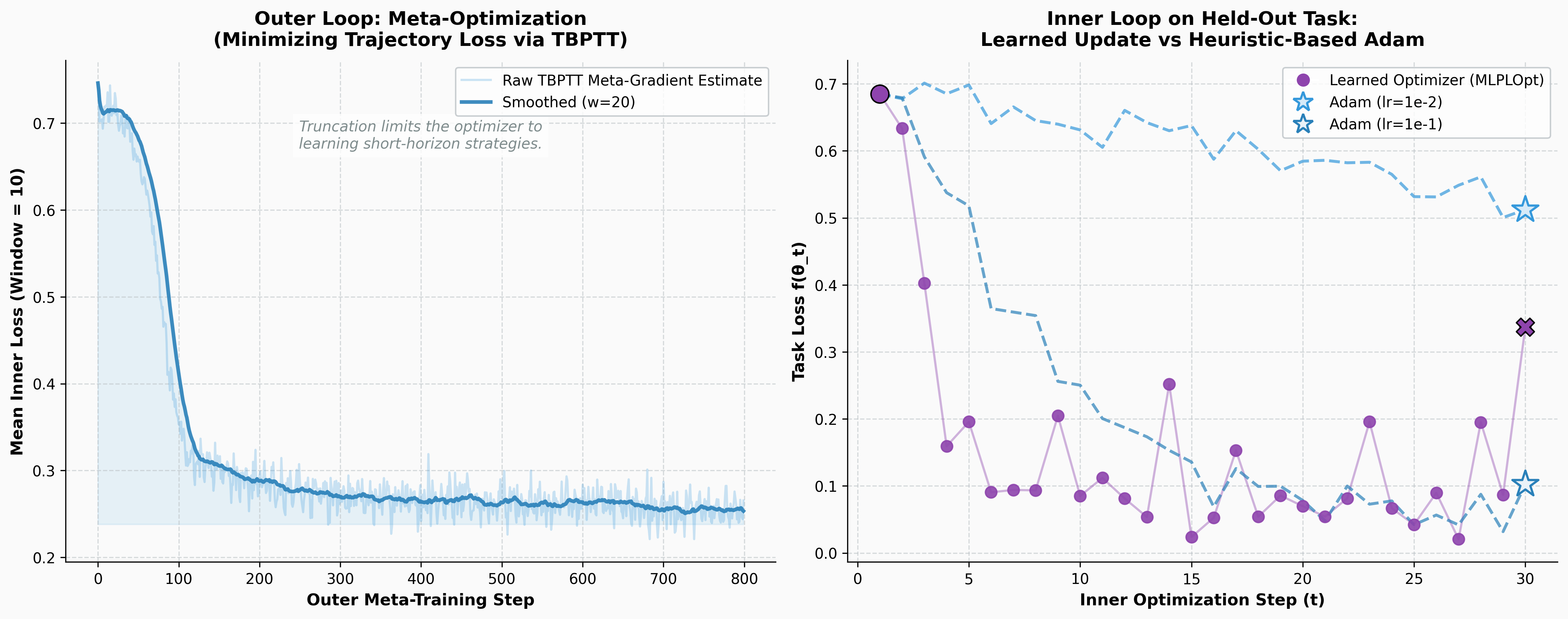 Left: The outer loop successfully minimizing the trajectory loss over 800 meta-training steps. Right: The inner loop on a completely unseen, held-out task. The learned optimizer exploits the landscape geometry to minimize the loss significantly faster than heuristic-based Adam.
While the JAX library is incredibly comprehensive for deep research, PyLO is much more recent and actively maintained. The fact that these infrastructures are being built is a great sign that the field is maturing beyond pure research curiosity.
Conclusion: The Future of Optimization
If learned optimizers are so good, why aren’t we all using torch.optim.LSTMOptimizer today?
The reality is that meta-learning an optimizer is computationally brutal. You are backpropagating through an entire training trajectory (Backpropagation Through Time). It’s incredibly memory-hungry and prone to extreme instability. While they proved it works on small models and specific domains like Neural Art styling, scaling this to train massive transformer models remains an open research challenge.
However, the core takeaway is undeniable. The Bitter Lesson is coming for optimizers, too. We are currently stuck in the “feature engineering” era of optimization. As compute grows and meta-learning stability improves, the idea of manually guessing eps=1e-8 or beta=(0.9, 0.999) will eventually seem just as archaic as hand-coding an edge detector in C++.
But we are not just waiting for more compute. The current training paradigm itself has structural limitations. If backpropagation through long optimization trajectories is unstable and biased, can we train optimizers without relying on it? I am still exploring the literature, but it seems there are several interesting alternatives out there. Some approaches appear to focus on local objectives that avoid unrolling entirely. Others seem to frame the problem using reinforcement learning techniques to bypass differentiable paths. I have also seen mentions of evolutionary and gradient-free methods gaining traction, alongside structure-aware optimizers that attempt to bridge the gap between diagonal and full-matrix preconditioners. I am still piecing all of this together, and I might write a follow-up post.
If you have made it this far and found this article useful, you can buy me a bag of tea/一包茶, it helps me keep writing posts like this one, as they’ve been taking more and more time :)) hopefully the quality shows off.
References
- Sutton, R. (2019). The Bitter Lesson.
- Andrychowicz, M., et al. (2016). Learning to learn by gradient descent by gradient descent. Advances in Neural Information Processing Systems.
- Metz, L., Maheswaranathan, N., Nixon, J., Freeman, C. D., & Sohl-Dickstein, J. (2018). Understanding and correcting pathologies in the training of learned optimizers. arXiv preprint arXiv:1810.10180.
- Metz, L., Freeman, C. D., Harrison, J., Maheswaranathan, N., & Sohl-Dickstein, J. (2022). Practical tradeoffs between memory, compute, and performance in learned optimizers. Conference on Lifelong Learning Agents (CoLLAs).
- Google Research. learned_optimization.
- Hugging Face. Ultrascale Playbook section on DDP compute communication overlap.
- Janson, P., Therien, B., Anthony, Q., Huang, X., Moudgil, A., & Belilovsky, E. (2025). PyLO: Towards Accessible Learned Optimizers in Pytorch.
Citation
If you found this work useful, please cite it as:
Klioui, S. (2026). Towards a Bitter Lesson of Optimization: When Neural Networks Write Their Own Update Rules
1
2
3
4
5
6
7
8
@article{klioui2026learnedopt,
  title   = {Towards a Bitter Lesson of Optimization: When Neural Networks Write Their Own Update Rules},
  author  = {Klioui, Sifal},
  journal = {Sifal Klioui Blog},
  year    = {2026},
  month   = {April},
  url     = {[https://sifal.social/posts/The-Bitter-Lesson-of-Optimization/](https://sifal.social/posts/The-Bitter-Lesson-of-Optimization/)}
}