Vanishing and exploding Gradients – A non-flat-earther's perspective.

Premise

As much as this post is about gradients, it’s also about having the confidence to fact check ourselves (or at the very least attempt to) about what we may consider as dogmatic truths, as by choosing not to, we become someone’s flat-earther.

Exploring the Impact of Activation Functions and Layer Normalization on Gradient Flow in Neural Networks

In this post I want us to explore how activation functions and layer normalization influence gradient flow and training efficiency in neural networks. Specifically, we’ll see how choices in these design elements affect the notorious vanishing gradient problem, which can severely impede model training. To illustrate this, we’ll run a series of experiments on a neural network trained on MNIST data, manipulating both the activation functions and normalization layers to observe their effects on gradients and convergence speed.

Background: Why Gradient Flow Matters

In training neural networks, gradients are central to updating weights. Through backpropagation, gradients flow backward from the output layer to each preceding layer, informing weight adjustments that minimize the loss. However, the gradients can sometimes become very small (the vanishing gradient problem) or excessively large (the exploding gradient problem) as they propagate. In deep networks, the vanishing gradient problem is especially pronounced when using sigmoid activation functions because these functions tend to diminish gradients, slowing or even halting learning in earlier layers.

To demonstrate this, we will manipulate the input normalization to bring the sigmoid activations closer to saturation. This amplifies the vanishing gradient effect, allowing us to examine how various configurations influence gradient flow.

Experiment Setup

Neural Network Architecture

We’ll use a simple, fully connected neural network with two layers:

1. Input Layer: Maps each 28x28 MNIST image (flattened to 784 values) to a hidden layer of 128 units.
2. Output Layer: Outputs 10 values corresponding to the 10 digit classes.

Each layer configuration will be adjusted to test different combinations of:

• Activation Functions: Sigmoid vs. ReLU
• Layer Normalization: With vs. without normalization

Experiment Configurations

To systematically test the impact of activation function and layer normalization on gradient flow, we define four experimental configurations:

• Experiment 1: Sigmoid activation, with layer normalization
• Experiment 2: Sigmoid activation, without layer normalization
• Experiment 3: ReLU activation, with layer normalization
• Experiment 4: ReLU activation, without layer normalization

This allows us to observe how each setup affects gradient dynamics, training performance, and convergence speed.

Key Normalization Adjustment

In this experiment, we normalize MNIST inputs differently from the typical approach. Instead of standardizing the values, we use transforms.Normalize((0.0,), (0.5,)) essentially scaling the inputs by a factor of 2. This adjustment pushes sigmoid outputs closer to their saturation point (near 1 or 0), resulting in very small gradients. This deliberate setup emphasizes the vanishing gradient problem, giving us a clear view of how normalization and activation choice impact gradient flow.

Sigmoid Activation and Vanishing Gradients

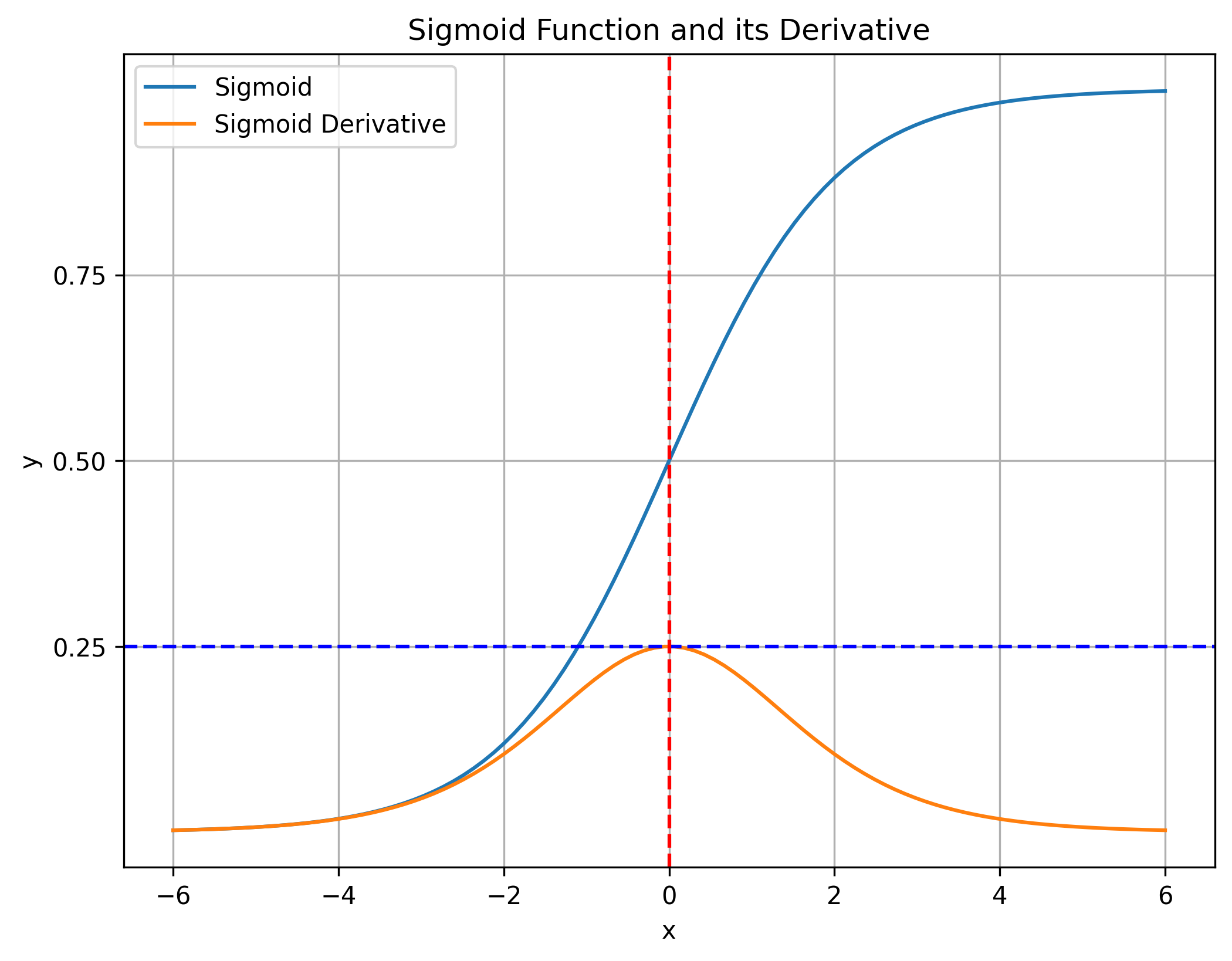
The sigmoid activation function is defined as:

\[\sigma(x) = \frac{1}{1 + e^{-x}}\]

Its derivative is:

\[\sigma'(x) = \sigma(x)(1 - \sigma(x))\]

The derivative of the sigmoid approaches zero for inputs far from zero (large positive or negative values), meaning that as gradients backpropagate through each sigmoid layer, they multiply by terms close to zero, shrinking rapidly.

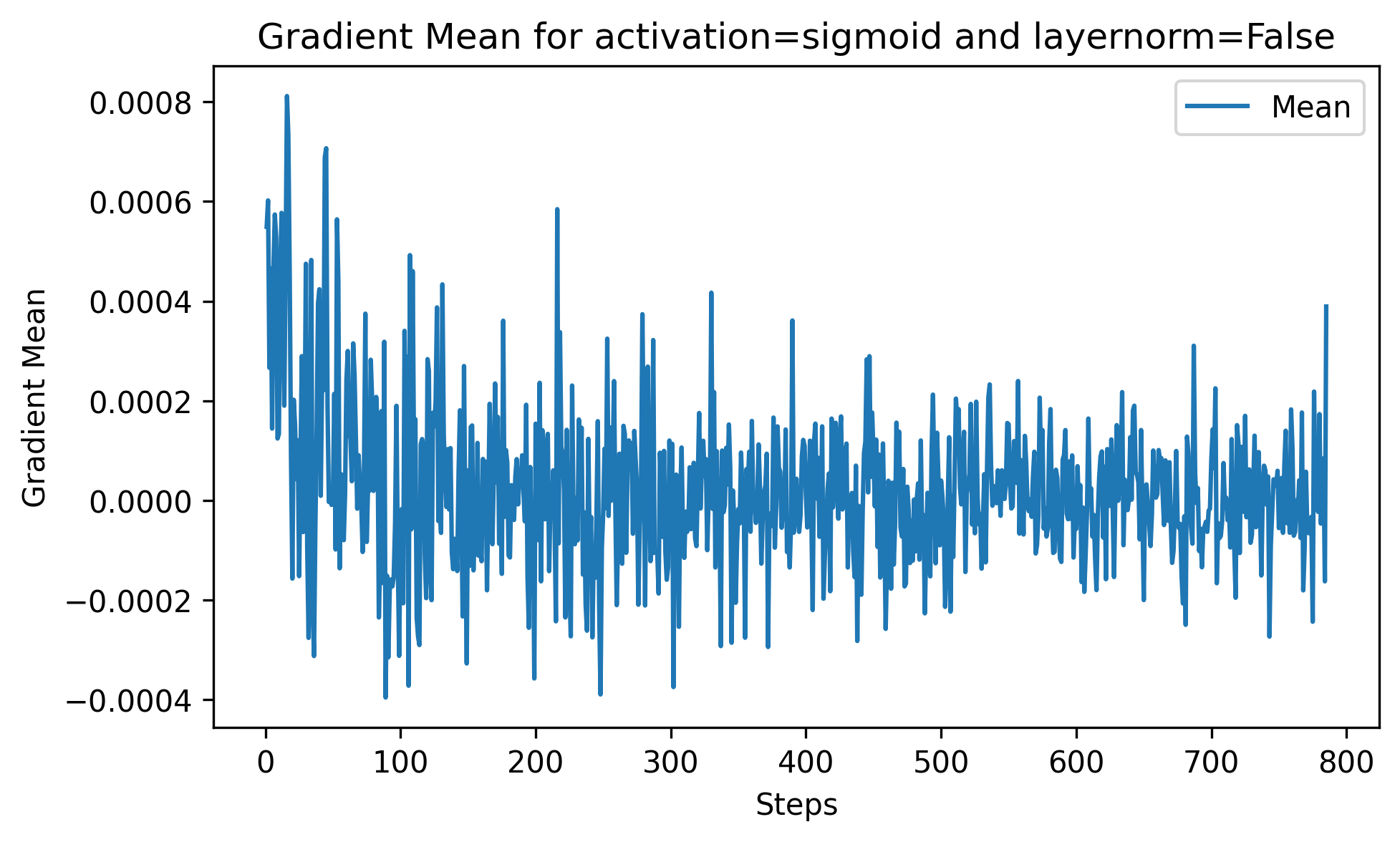
The following figure below clearly shows how gradient vanishing happens as the \(\mid mean \mid\) is mostly on average 2e-4, and most importantly it starts at extremely small values! This shouldn’t be the case because a lot of the learning that happens in the first steps is generally considered the easiest. These small gradient leads to very small updates during the optimization, and the convergences becomes either extremely slow or simply impossible.

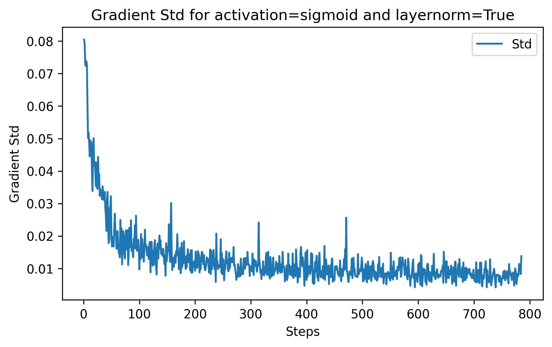
Now let’s see what happens when we feed the inputs to a layer-norm.

The gradients are much better! 2 order of magnitude more than before, and on average they starts at 8e-2! (Note that it usually natural for the gradients to decrease as the learning goes)

ReLU Activation as an Alternative

Now let’s talk about ReLU activation which is defined as:

\[\text{ReLU}(x) = \max(0, x), \quad \text{ReLU}'(x) = \begin{cases} 1 & \text{if } x > 0 \\ 0 & \text{if } x \leq 0 \end{cases}\]

Since ReLU’s derivative is either 1 or 0, it does not suffer from vanishing gradients for positive values. However, it can still lead to dead neurons if inputs remain negative. But this time we will see how it can lead to the opposite effect i.e exploding gradients: when the inputs are big the ReLU doesn’t not have the ability to ‘squeeze’ them, thus leading to big activations, the effect here is that the optimization step that are taken are too big, leading to a sort of ping pong in the loss curvature.

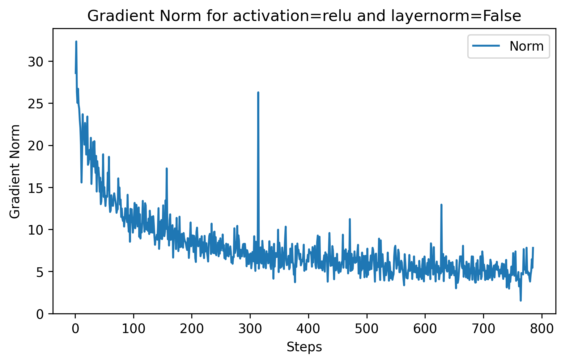
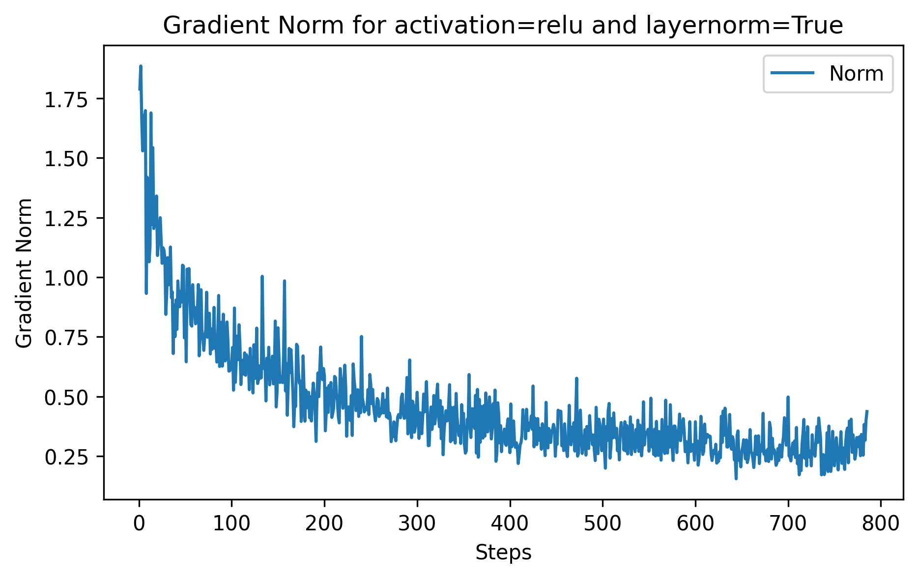
Another way to visualize the effect of vanishing/exploding gradients is to track their l2 norm (essentially the length of the vector):

When we apply the layer norm to the inputs, we can see a directly see a direct impact on the norm, it noticeably reduces it, and it also has the effect of avoiding the spikes like we can see in ~step 300 without layer norm

The Mathematics of Gradient Flow: The Chain Rule

Now let’s dig into some math, in neural networks, gradients propagate backward through each layer according to the chain rule. For a neural network with multiple layers, the chain rule multiplies the derivatives from each layer, producing the final gradient for each weight.

In our case, a two-layer network with sigmoid activation in the hidden layer would have gradients of the following form:

\[\frac{\partial L}{\partial \mathbf{W}^{[1]}} = \frac{\partial L}{\partial a^{[2]}} \cdot \frac{\partial a^{[2]}}{\partial z^{[2]}} \cdot \frac{\partial z^{[2]}}{\partial a^{[1]}} \cdot \frac{\partial a^{[1]}}{\partial z^{[1]}} \cdot \frac{\partial z^{[1]}}{\partial \mathbf{W}^{[1]}}\]

This chain rule multiplication means that each layer’s gradient depends on the gradients of the layers after it. If any of these terms are very small, such as in layers with the sigmoid activation function, the entire gradient for earlier layers will shrink, leading to the vanishing gradient problem.

Why Normalization Helps

By normalizing inputs, we keep the values within a range where the sigmoid derivative is significant. This helps gradients retain their magnitude. For example, layer normalization centers and scales the activations at each layer to prevent activations from saturating, allowing gradients to propagate more effectively through sigmoid layers.

Results and Key Takeaways

We observe the following:

• Sigmoid without layer normalization results in vanishing gradients due to saturation.
• Sigmoid with layer normalization mitigates this effect but still has smaller gradients compared to ReLU.
• ReLU without normalization allows larger gradients but may lead to dead neurons.
• ReLU with normalization provides the most stable and efficient gradient flow.

This experiment demonstrates why input normalization and activation choice are essential for effective training. By using the chain rule and understanding the mathematics behind gradients, we can design networks that avoid common pitfalls like the vanishing gradient problem, making training faster and more stable.

Flat earther detector

If you’ve come this far then I hope you’ve learned a few things!

I’ve deliberately ignored an element that is essential to truthfully describe the effects that we’ve learned about, can you figure out what it is, and prove to yourself that you’re not a flat eather?

Code and Gradient Tracking

You can use the following code to track gradient statistics for each layer. This includes the mean and norm of the gradients to evaluate the behavior across configurations.

# Import necessary libraries
import torch
import torch.nn as nn
import torch.nn.functional as F
import torch.optim as optim
from torchvision import datasets, transforms
from tqdm.auto import tqdm
import numpy as np
import matplotlib.pyplot as plt

# Define the neural network
class Net(nn.Module):
    def __init__(self, apply_layer_norm=True, activation='sigmoid'):
        super(Net, self).__init__()
        self.fc1 = nn.Linear(784, 128)
        self.fc2 = nn.Linear(128, 10)
        self.apply_layer_norm = apply_layer_norm
        if apply_layer_norm:
            self.ln = nn.LayerNorm(128)
        self.activation = nn.Sigmoid() if activation == 'sigmoid' else nn.ReLU()
        
    def forward(self, x):
        x = torch.flatten(x, 1)
        x = self.fc1(x)
        if self.apply_layer_norm:
            x = self.ln(x)
        x = self.activation(x)
        return F.log_softmax(self.fc2(x), dim=1)

# Function to log gradient statistics
def track_gradient_statistics(model):
    grad_stats = {}
    for name, param in model.named_parameters():
        if param.requires_grad and param.grad is not None:
            grad_stats[name] = {
                'mean': param.grad.mean().item(),
                'std': param.grad.std().item(),
                'norm': param.grad.norm().item()
            }
    return grad_stats

# Training function to log gradient stats per configuration
def train(model, device, train_loader, optimizer, epoch, grad_stats_list):
    model.train()
    for batch_idx, (data, target) in enumerate(train_loader):
        data, target = data.to(device), target.to(device)
        optimizer.zero_grad()
        output = model(data)
        loss = F.nll_loss(output, target)
        loss.backward()
        
        # Track gradient statistics
        grad_stats = track_gradient_statistics(model)
        grad_stats_list.append(grad_stats)
        
        optimizer.step()

# Setup data loader with custom normalization to amplify sigmoid's vanishing gradient effect
train_loader = torch.utils.data.DataLoader(
    datasets.MNIST('./data', train=False, download=True,
                   transform=transforms.Compose([
                       transforms.ToTensor(),
                       transforms.Normalize((0.0,), (0.5,))  # Multiplies inputs by 2
                   ])),
    batch_size=64, shuffle=True)