Why Modern LLMs Dropped Mean Centering (And Got Away With It)

Every major modern LLM has quietly dropped one of the two steps that define standard Layer Normalization. They removed mean centering. And it works. Why?

The standard answer is “it’s cheaper and empirically fine.” But that’s unsatisfying. If mean centering exists for a reason, removing it must have consequences. What are they, exactly? And does RMSNorm secretly recover what it gave up?

Those questions don’t have clean answers if you only look at the algebra. But if you look at the geometry, everything snaps into place. When we strip away the indices and summations, normalization turns out to be a beautiful sequence of spatial transformations: projections onto planes, locking data to hyperspheres, stretching those spheres into ellipsoids. Operations that look like statistical bookkeeping are actually sculpting the shape of your activation space.

My goal here is to make this visually intuitive, the kind of intuitive where you can close your eyes and watch the data move. I’ve built a 3D toy simulation showing exactly what happens at each step of standard LayerNorm, including the surprisingly consequential effect of the $\epsilon$ parameter (yes, $\epsilon$ again, I wrote about it trapping the Adam optimizer, and here it is causing trouble again :O).

More importantly, I want to share a derivation I haven’t seen covered elsewhere: a unified formulation that shows exactly how RMSNorm relates to standard LayerNorm, both mathematically and geometrically. The result reframes RMSNorm not as a cheaper approximation, but as a self-regulating system with two distinct behavioral modes depending on the health of your network.

The geometric foundations here were laid by Andy Arditi’s notes and Paul M. Riechers’ paper Geometry and Dynamics of LayerNorm, both well worth reading. This post builds on that work and adds the RMSNorm piece.

Let’s jump in.

1. The Anatomy of LayerNorm

Given an activation vector $\vec{x} \in \mathbb{R}^n$, the standard LayerNorm operation is defined as:

\[LayerNorm(\vec{x}) = \vec{g} \odot \frac{\vec{x} - \mu_{\vec{x}}}{\sqrt{\sigma_{\vec{x}}^2 + \epsilon}} + \vec{b}\]

We can break this down into three distinct geometric phases.

Phase 1: Mean Centering (The Orthogonal Complement)

Let’s start with the intuition. What happens when you subtract the mean from a set of numbers? By definition, the sum of those new, centered elements becomes exactly zero.

Mathematically, summing the elements of a vector is equivalent to performing a dot product with a vector of all ones ($\vec{1}$). So, if the sum of our centered vector is zero, its dot product with $\vec{1}$ must also be zero.

Just a quick reminder: when the dot product of two non-zero vectors is zero, it means they are perfectly perpendicular (orthogonal) to each other.

This tells us that the mean-centered data is orthogonal to the vector of ones. So, while $\vec{x}^{(1)} = \vec{x} - \mu_{\vec{x}}$ looks like a simple statistical shift, geometrically, it’s a projection. By subtracting the mean, we are taking our data vector and stripping away its “shadow” along the diagonal axis of the space. \(\vec{x}^{(1)} = \vec{x} - (\vec{x} \cdot \hat{1})\hat{1}\)

Algebraic Equivalence: Mean Centering as an Orthogonal Projection.

We want to show that subtracting the mean is equivalent to subtracting the vector's projection onto the unit vector of ones ($\hat{1}$). The standard formula for the mean is: $$ \mu_{\vec{x}} = \frac{1}{n} \sum_{i=1}^n x_i = \frac{1}{n}(\vec{x} \cdot \vec{1}) $$ We define the unit vector $\hat{1}$ by dividing the vector of ones by its length ($\sqrt{n}$): $$ \hat{1} = \frac{\vec{1}}{\sqrt{n}} \implies \vec{1} = \sqrt{n}\hat{1} $$ Now, substitute this into a vector representing the mean shifted across all dimensions ($\mu_{\vec{x}}\vec{1}$): $$ \mu_{\vec{x}}\vec{1} = \frac{1}{n}(\vec{x} \cdot \sqrt{n}\hat{1})(\sqrt{n}\hat{1}) $$ Pulling the scalars out to the front gives: $$ \mu_{\vec{x}}\vec{1} = \frac{n}{n}(\vec{x} \cdot \hat{1})\hat{1} = (\vec{x} \cdot \hat{1})\hat{1} $$ Thus, subtracting the mean is mathematically identical to subtracting the orthogonal projection onto $\hat{1}$: $$ \vec{x}^{(1)} = \vec{x} - \mu_{\vec{x}}\vec{1} = \vec{x} - (\vec{x} \cdot \hat{1})\hat{1} $$

By definition, taking a vector and removing its projection along a line forces the result to live in the space perpendicular to that line. We are projecting our $n$-dimensional activations onto an $(n-1)$-dimensional flat plane (the orthogonal complement of $\vec{1}$).

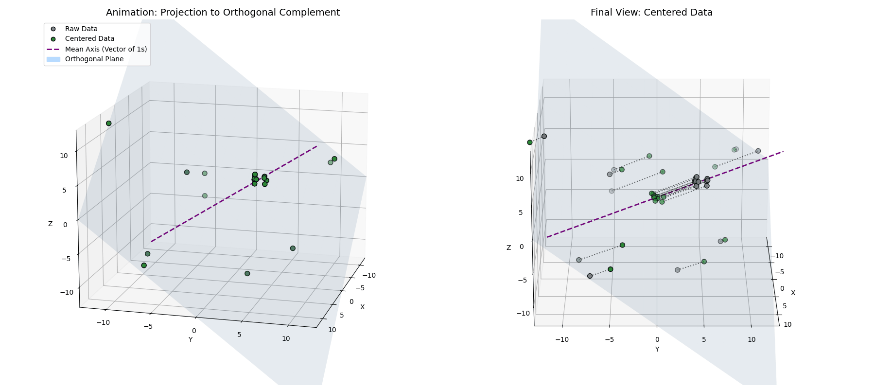Notice how the data (blue) is projected straight down onto the cyan plane (where $x+y+z=0$), resulting in the centered points (crimson).

Phase 2: Variance Normalization (The Hypersphere)

Now for the variance. Intuitively, dividing by the standard deviation forces all our data vectors to have a consistent spread.

It feels incredibly natural to assume that dividing by this deviation projects the vector onto a unit sphere (a sphere with a radius of 1). But this is a mathematical illusion!

To project a vector onto a unit sphere (radius 1), you must divide it by its exact geometric length (the L2 norm, $\lVert\vec{x}\rVert$)

Standard deviation ($\sigma$) isn’t the geometric length! Because variance is the average of the squared distances ($\sigma^2 = \frac{1}{n}\lVert\vec{x}^{(1)}\rVert^2$), dividing by $\sigma$ actually projects our data onto a hypersphere of a much larger radius, specifically $\sqrt{n}$. \(\vec{x}^{(2)} = \sqrt{n} \frac{\vec{x}^{(1)}}{||\vec{x}^{(1)}||}\)

Radius Proof: Why Normalization Targets the $\sqrt{n}$ Hypersphere.

We want to prove that dividing by the standard deviation scales a vector to a length of exactly $\sqrt{n}$. The variance of our mean-centered vector is the average of its squared components: $$ \sigma_{\vec{x}}^2 = \frac{1}{n} \sum_{i=1}^n (x_i^{(1)})^2 = \frac{1}{n} ||\vec{x}^{(1)}||^2 $$ Taking the square root gives us the standard deviation: $$ \sigma_{\vec{x}} = \frac{1}{\sqrt{n}} ||\vec{x}^{(1)}|| $$ When we perform the normalization step ($\vec{x}^{(2)} = \frac{\vec{x}^{(1)}}{\sigma_{\vec{x}}}$), we substitute the definition of $\sigma_{\vec{x}}$: $$ \vec{x}^{(2)} = \frac{\vec{x}^{(1)}}{\frac{1}{\sqrt{n}} ||\vec{x}^{(1)}||} = \sqrt{n} \frac{\vec{x}^{(1)}}{||\vec{x}^{(1)}||} $$

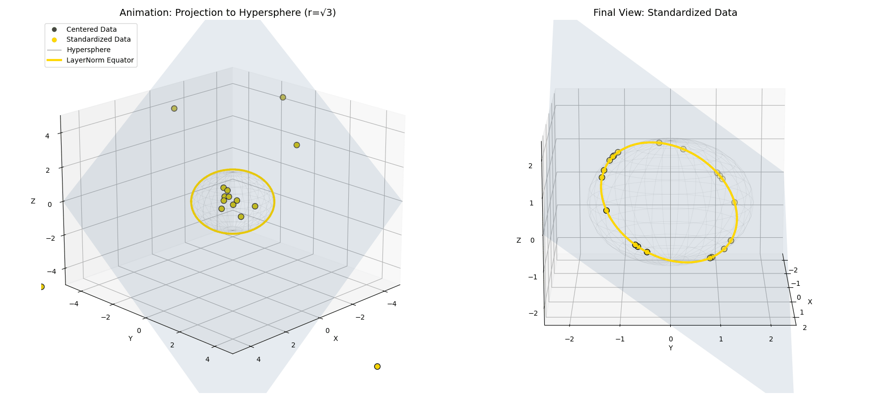The mean-centered points (green) are radially pushed or pulled until they lock onto the intersection of the flat plane and a hypersphere of radius $\sqrt{n}$ (the red ring).

Phase 3: The Affine Transformation ($\gamma$ and $\beta$)

We just spent all that compute forcing our data onto a perfectly rigid, predictable spherical ring. Why? So the neural network can safely warp it into whatever shape it actually needs to learn!

The learned parameters $\vec{g}$ (often called $\gamma$) and $\vec{b}$ (often called $\beta$) apply an affine transformation:

\[\vec{x}^{(3)} = \vec{g} \odot \vec{x}^{(2)} + \vec{b}\]

Because $\vec{g}$ is applied via element-wise multiplication ($\odot$), it stretches our perfect sphere unevenly along the different feature axes, transforming the hypersphere into a hyper-ellipsoid. Then, adding the bias $\vec{b}$ simply picks up that ellipsoid and translates it through space.

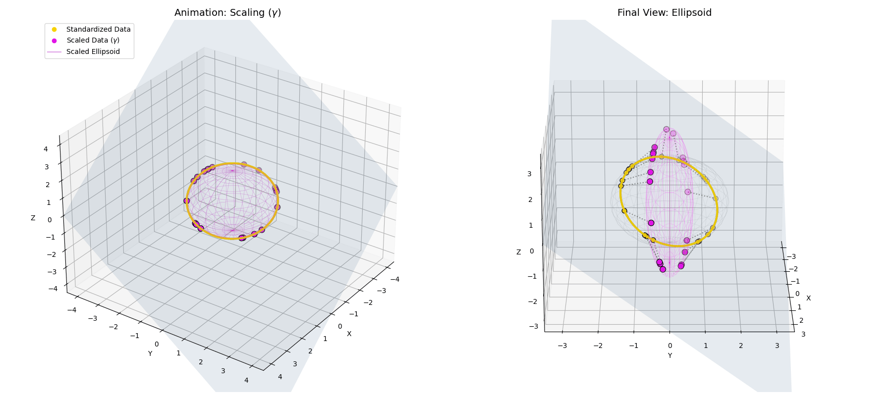The $\gamma$ parameter stretches the perfect spherical ring into an elliptical shape, scaling different feature dimensions based on their learned importance.

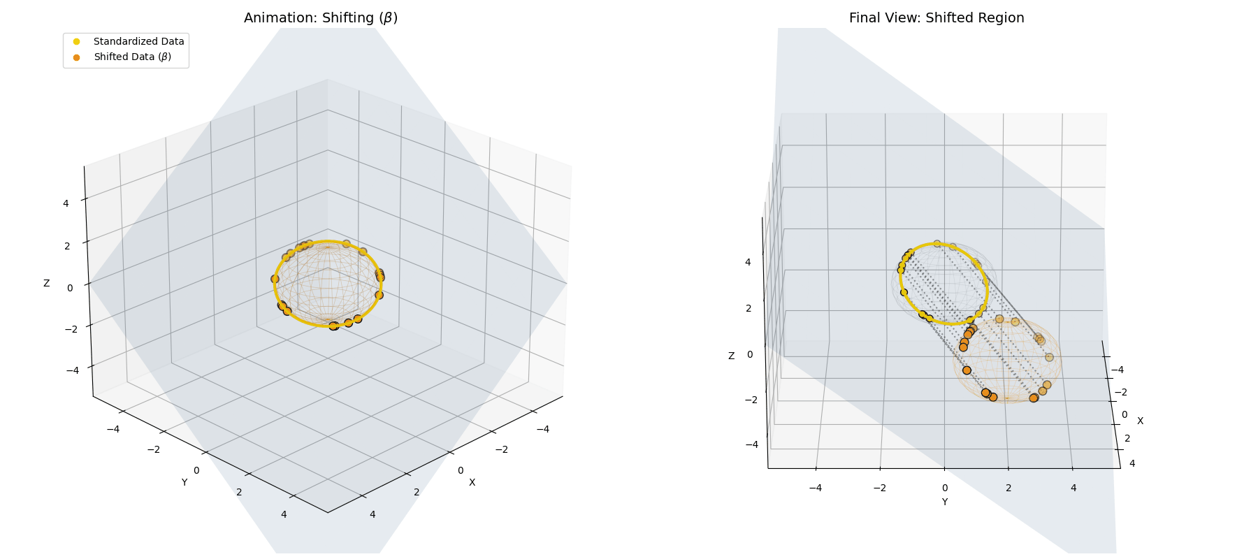The $\beta$ parameter simply translates the entire newly formed ellipsoid to a new center of gravity in the latent space.

The $\epsilon$ Anomaly: A Solid Ball, Not a Hollow Shell

Let’s think about this intuitively: if you divide a number by something slightly larger than itself, the result is always less than 1.

In the denominator of LayerNorm, there is a tiny constant $\epsilon$ (usually $10^{-5}$) added for numerical stability to prevent division by zero.

By adding a positive $\epsilon$, the denominator ($\sqrt{\sigma_{\vec{x}}^2 + \epsilon}$) becomes strictly larger than the true standard deviation.

Because of this geometric trick, the denominator is always slightly larger than the true variance:

\[||\vec{x}^{(2)}|| = \sqrt{n} \left( \frac{||\vec{x}^{(1)}||}{\sqrt{||\vec{x}^{(1)}||^2 + n\epsilon}} \right)\]

The Epsilon Effect: Deriving the Pull Toward the Origin

We want to see how adding $\epsilon$ alters the final length of our normalized vector. We start with the normalization equation including $\epsilon$: $$ \vec{x}^{(2)} = \frac{\vec{x}^{(1)}}{\sqrt{\sigma_{\vec{x}}^2 + \epsilon}} $$ Let's find the magnitude (norm) of this new vector: $$ ||\vec{x}^{(2)}|| = \frac{||\vec{x}^{(1)}||}{\sqrt{\sigma_{\vec{x}}^2 + \epsilon}} $$ Substitute our definition of variance ($\sigma_{\vec{x}}^2 = \frac{1}{n}\lVert\vec{x}^{(1)}\rVert^2$) into the denominator: $$ ||\vec{x}^{(2)}|| = \frac{||\vec{x}^{(1)}||}{\sqrt{\frac{1}{n}||\vec{x}^{(1)}||^2 + \epsilon}} $$ To simplify, factor $\frac{1}{n}$ out from the terms inside the square root: $$ \sqrt{\frac{1}{n} (||\vec{x}^{(1)}||^2 + n\epsilon)} = \frac{1}{\sqrt{n}} \sqrt{||\vec{x}^{(1)}||^2 + n\epsilon} $$ Substitute this back into the denominator, bringing the $\sqrt{n}$ up to the numerator: $$ ||\vec{x}^{(2)}|| = \sqrt{n} \left( \frac{||\vec{x}^{(1)}||}{\sqrt{||\vec{x}^{(1)}||^2 + n\epsilon}} \right) $$

This means the data never actually reaches the surface of the $\sqrt{n}$ sphere.

Furthermore, because LayerNorm calculates a different variance for every single token, $\epsilon$ pulls on them unevenly:

• “Loud” Data (High Variance): The signal dwarfs $\epsilon$, so the fraction is basically 1. The point lands right on the inside surface of the sphere.
• “Quiet” Data (Low Variance): The signal is tiny, so the $n\epsilon$ constant dominates the denominator. The point is violently pulled inward toward the origin.

Because of $\epsilon$, LayerNorm doesn’t project data onto a hollow, razor-thin shell. It projects data into a solid ball, with points distributed radially based on their original variance!

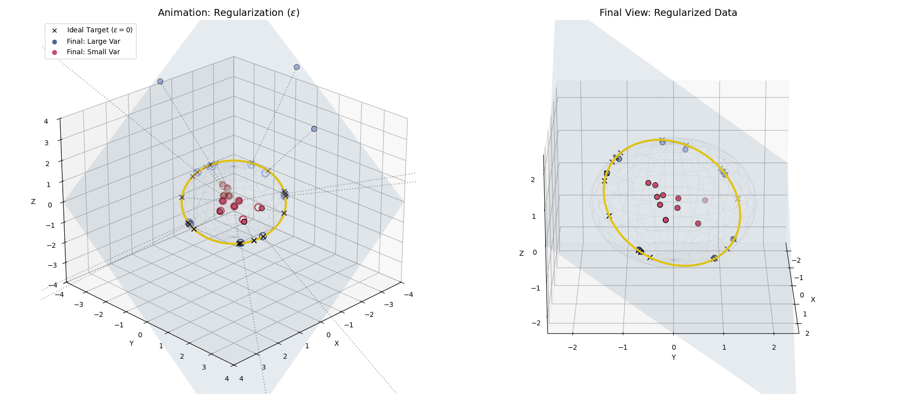With $\epsilon$ applied, large variance points (blue) hit the target ring, while small variance points (red) fall short, getting trapped closer to the origin.

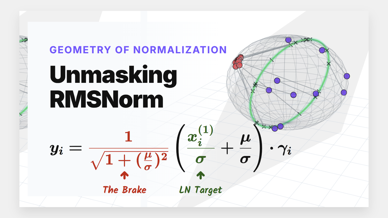
The Main Event: Unmasking RMSNorm

Modern LLMs have largely abandoned standard LayerNorm in favor of RMSNorm (Root Mean Square Normalization).

Let’s start with the intuition again. Why would we ever drop the mean centering? Deep neural networks tend to have activations with a mean that naturally hovers close to zero anyway. If the mean is already tiny, explicitly calculating and subtracting it over and over is just a waste of compute.

RMSNorm gambles on the assumption that the variance (the “signal” spread) will almost always dominate the mean (the “noise” shift).

RMSNorm completely drops the mean-centering step, simplifying the formula to:

\[RMSNorm(\vec{x}) = \vec{g} \odot \frac{\vec{x}}{\sqrt{\frac{1}{n}\sum x_i^2}}\]

But wait. If we skip mean-centering, aren’t we destroying the elegant geometry we just built? How does this actually relate to standard LayerNorm?

Here’s the key insight: every raw input $x_i$ can always be decomposed as $x_i = x_i^{(1)} + \mu$, where $x_i^{(1)}$ is the mean-centered version and $\mu$ is the mean. This is trivially true, it’s just adding and subtracting the mean. But the point is that this decomposition lets us surgically expose what RMSNorm is ignoring by skipping the centering step, and quantify exactly how large that gap is as a function of the mean-to-variance ratio.

To find out, I substituted this decomposition into the RMSNorm equation. The denominator, which starts as $\sqrt{\frac{1}{n}\sum x_i^2}$, expands via the cross terms and then collapses beautifully: the middle term vanishes because the sum of mean-centered values is zero by definition, leaving the denominator as $\sqrt{\sigma^2 + \mu^2}$.

Unified Formulation: Decomposing RMSNorm into Signal and Noise.

We want to show how RMSNorm mathematically simplifies when we explicitly expose the mean and variance. We start with the standard RMSNorm definition: $$ y_i = \frac{x_i}{RMS(\vec{x})} * \gamma_i \quad \text{where} \quad RMS(\vec{x}) = \sqrt{\frac{1}{n}\sum_{j=1}^n x_j^2} $$ We introduce the transformation to separate the mean-centered input from the mean: $x_j = x_j^{(1)} + \mu$. Because it's mean-centered, the sum of the mean-centered inputs is zero ($\sum_{j=1}^n x_j^{(1)} = 0$). We also know that the variance $\sigma^2$ is the mean of the squared mean-centered inputs ($\sigma^2 = \frac{1}{n}\sum_{j=1}^n (x_j^{(1)})^2$). Replace the raw input $x_j$ with the transformed version inside the square root and expand using the binomial theorem: $$ RMS(\vec{x}) = \sqrt{\frac{1}{n}\sum_{j=1}^n \left( (x_j^{(1)})^2 + 2x_j^{(1)}\mu + \mu^2 \right)} $$ Split the equation into three separate sums: $$ RMS(\vec{x}) = \sqrt{\frac{1}{n}\sum_{j=1}^n (x_j^{(1)})^2 + \frac{2\mu}{n}\sum_{j=1}^n x_j^{(1)} + \frac{1}{n}\sum_{j=1}^n \mu^2} $$ The middle term contains $\sum_{j=1}^n x_j^{(1)}$, which is 0. The entire middle term vanishes. The last term sums the constant $\mu^2$ exactly $n$ times, resulting in $n\mu^2$. Dividing by $n$ leaves just $\mu^2$: $$ RMS(\vec{x}) = \sqrt{\frac{1}{n}\sum_{j=1}^n (x_j^{(1)})^2 + \mu^2} $$ Recognizing the remaining summation is exactly the definition of variance ($\sigma^2$), we get: $$ RMS(\vec{x}) = \sqrt{\sigma^2 + \mu^2} $$ To isolate the ratio of the mean to the standard deviation, we factor $\sigma^2$ out of the terms inside the square root: $$ RMS(\vec{x}) = \sqrt{\sigma^2 \left( 1 + \frac{\mu^2}{\sigma^2} \right)} = \sigma\sqrt{1 + \left(\frac{\mu}{\sigma}\right)^2} $$ Now, return to the original RMSNorm equation ($y_i$). Substitute the transformed input ($x_i^{(1)} + \mu$) into the numerator, and our newly derived expression into the denominator: $$ y_i = \frac{x_i^{(1)} + \mu}{\sigma\sqrt{1 + (\frac{\mu}{\sigma})^2}} * \gamma_i $$ Factor out the square root portion, and separate the numerator over the standard deviation ($\sigma$) to explicitly show the LayerNorm component and the dynamic bias component: $$ y_i = \frac{1}{\sqrt{1 + (\frac{\mu}{\sigma})^2}} \left( \frac{x_i^{(1)}}{\sigma} + \frac{\mu}{\sigma} \right) * \gamma_i $$

If we substitute this back into the full equation and separate the terms, we get a beautiful, unified formulation of RMSNorm:

\[y_i = \frac{1}{\sqrt{1 + (\frac{\mu}{\sigma})^2}} \left( \frac{x_i^{(1)}}{\sigma} + \frac{\mu}{\sigma} \right) * \gamma_i\]

This equation is a goldmine. It proves that RMSNorm is mathematically identical to standard LayerNorm, just modulated by a dynamic “signal-to-noise” ratio ($\mu/\sigma$).

Let’s look at the three pieces:

1. The LayerNorm Core: $\frac{x_i^{(1)}}{\sigma}$ is exactly standard LayerNorm.
2. The Dynamic Bias: $\frac{\mu}{\sigma}$ acts as an automatic, data-dependent shift.
3. The Dampening Factor: $\frac{1}{\sqrt{1 + (\mu/\sigma)^2}}$ acts as an automatic brake.

This formulation dictates two distinct behavioral regimes for our models.

Case 1: The Healthy Network ($\sigma \gg |\mu|$)

In a well-behaved Transformer, the standard deviation of activations is naturally much larger than the mean.

If $\sigma$ dominates $\mu$, the ratio $\frac{\mu}{\sigma}$ approaches 0. Look at what happens to our equation: The dampening factor becomes $\frac{1}{\sqrt{1+0}} = 1$, and the dynamic bias vanishes.

RMSNorm closely approximates standard LayerNorm. It doesn’t land exactly on the perfect LayerNorm target equator because we completely skipped the explicit centering step. However, because the standard deviation is so large, the data is widely spread out and lands very close to that ideal $\sqrt{n}$ spherical ring, achieving a highly similar geometric goal while saving compute.

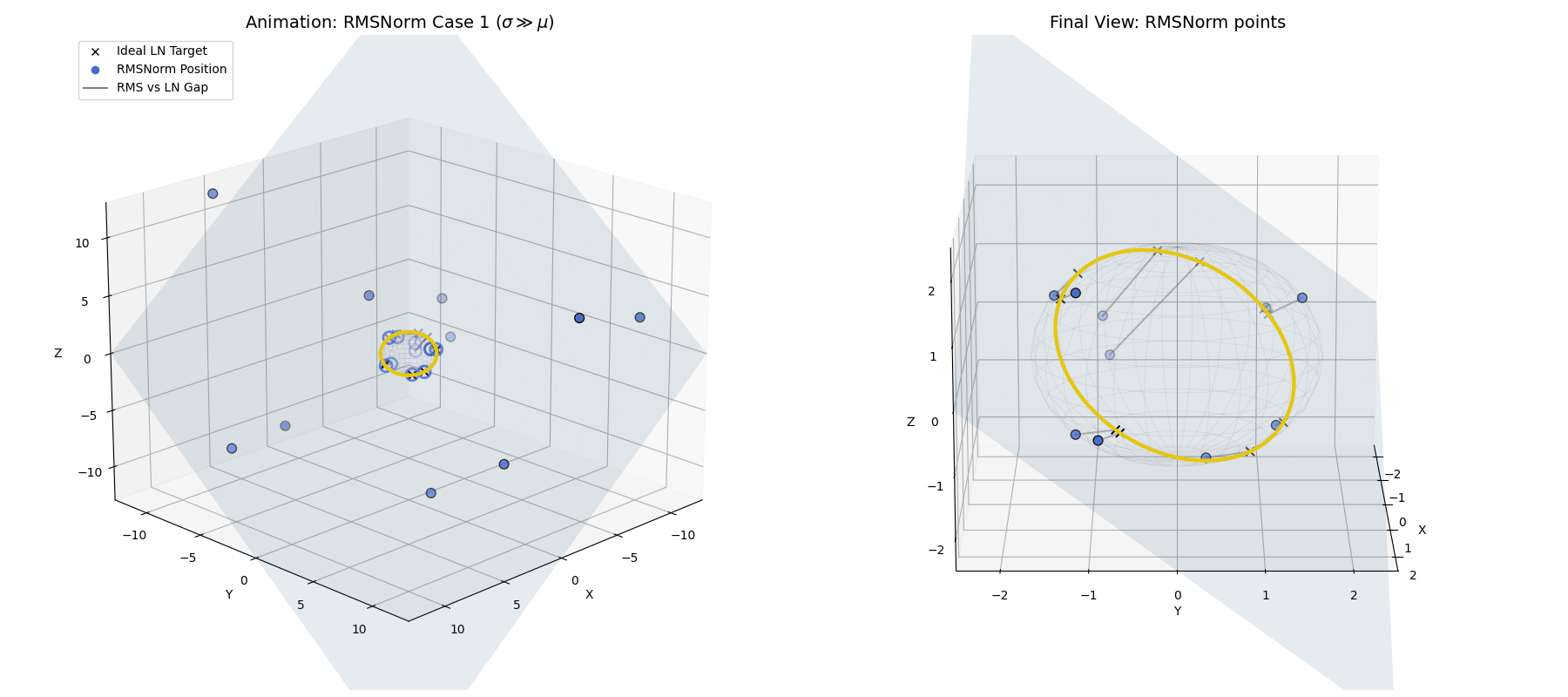When $\sigma \gg \mu$, the raw data (blue dots) is naturally projected by RMSNorm to a spread-out ring that is very close to the exact LayerNorm target, without needing the explicit centering step.

Case 2: The Unstable Network ($\mu \gg \sigma$)

What if the network spikes and the mean violently drifts away from zero?

In standard LayerNorm, the explicit mean subtraction would blindly correct this. RMSNorm doesn’t have that luxury. Instead, as $|\mu|$ grows, the ratio $(\mu/\sigma)^2$ explodes.

Crucially, the output still lands on the $\sqrt{n}$ sphere (i.e., the L2 norm of the RMSNorm output is always $\sqrt{n}$ regardless of the input.)

Magnitude Invariance: Proving the Output Length is Always $\sqrt{n}$.

We want to show that $\lVert\text{RMSNorm}(\vec{x})\rVert = \sqrt{n}$ for any input $\vec{x}$, regardless of its mean or variance. First, observe that $RMS(\vec{x})$ is simply the L2 norm of $\vec{x}$ scaled by $\frac{1}{\sqrt{n}}$: $$ RMS(\vec{x}) = \sqrt{\frac{1}{n}\sum_{i=1}^n x_i^2} = \sqrt{\frac{1}{n}||\vec{x}||^2} = \frac{||\vec{x}||}{\sqrt{n}} $$ Now substitute this into the norm of the RMSNorm output (ignoring $\vec{g}$ for clarity, i.e. $\vec{g} = \vec{1}$): $$ \left|\left|\frac{\vec{x}}{RMS(\vec{x})}\right|\right| = \frac{||\vec{x}||}{RMS(\vec{x})} = \frac{||\vec{x}||}{\frac{||\vec{x}||}{\sqrt{n}}} = \sqrt{n} $$ The $\lVert\vec{x}\rVert$ terms cancel exactly, leaving $\sqrt{n}$ unconditionally. This means RMSNorm always projects onto the hypersphere of radius $\sqrt{n}$ ( the same target as standard LayerNorm ) regardless of the mean-to-variance ratio. What changes between the healthy ($\sigma \gg \mu$) and unstable ($\mu \gg \sigma$) regimes is not the magnitude of the output, but its $\textbf{direction}$.

What changes is not the magnitude but the direction. As $|\mu/\sigma| \to \infty$, the dampening factor approaches $\sigma/|\mu|$ and the per-token variation in $x_i^{(1)}/\sigma$ becomes negligible next to $\mu/\sigma$. Every point collapses toward the same location: $\text{sign}(\mu) \cdot \vec{\gamma}$.

The Limit of Diversity: Deriving Directional Collapse in Unstable Networks.

We want to show what the unified RMSNorm formulation converges to as $\|\mu/\sigma\| \to \infty$. Starting from our unified formulation: $$ y_i = \frac{1}{\sqrt{1 + \left(\frac{\mu}{\sigma}\right)^2}} \left( \frac{x_i^{(1)}}{\sigma} + \frac{\mu}{\sigma} \right) \gamma_i $$ As $|\mu/\sigma| \to \infty$, the 1 inside the square root becomes negligible: $$ \frac{1}{\sqrt{1 + \left(\frac{\mu}{\sigma}\right)^2}} \to \frac{1}{\sqrt{\left(\frac{\mu}{\sigma}\right)^2}} = \frac{1}{\left|\frac{\mu}{\sigma}\right|} = \frac{\sigma}{|\mu|} $$ Note that we take the absolute value because the square root always returns a non-negative result. As $|\mu/\sigma| \to \infty$, the centered term $x_i^{(1)}/\sigma$ is bounded (it depends only on the within-token variation, not on $\mu$), so it becomes negligible next to $\mu/\sigma$: $$ \frac{x_i^{(1)}}{\sigma} + \frac{\mu}{\sigma} \to \frac{\mu}{\sigma} $$ Multiplying the two limits together: $$ y_i \to \frac{\sigma}{|\mu|} \cdot \frac{\mu}{\sigma} \cdot \gamma_i = \frac{\mu}{|\mu|} \cdot \gamma_i = \text{sign}(\mu) \cdot \gamma_i $$ The input-specific information in $x_i^{(1)}$ vanishes entirely. Every token ( regardless of its actual values ) converges to the same point on the sphere, determined solely by the sign of the mean drift and the learned scale $\vec{\gamma}$. Positive mean drift collapses all tokens to one pole; negative drift collapses them to the antipodal pole.

Geometrically, this means RMSNorm maps all highly-shifted tokens to one of two antipodal poles on the sphere : the positive pole when the mean drifts upward, the negative pole when it drifts downward. The tokens don’t lose energy; they lose discriminability. Inputs that were genuinely different become nearly indistinguishable in the output, starving the subsequent attention layers of the directional diversity they need.

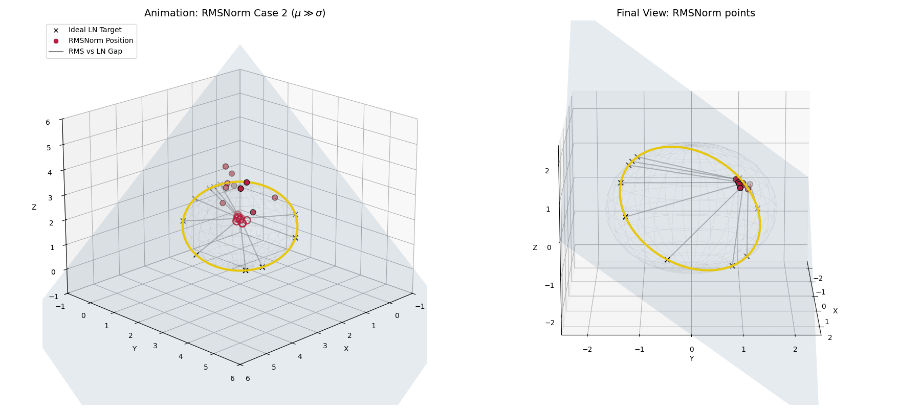When $\mu \gg \sigma$, RMSNorm (crimson dots) doesn’t correct the shift. All points still land on the $\sqrt{n}$ sphere, but they collapse toward the same pole, losing the directional diversity that LayerNorm would have preserved.

The Big Picture: RMSNorm vs LayerNorm

To really hammer this home, let’s look at a side-by-side comparison where both populations live together, similar to what we saw with the effect of epsilon.

RMSNorm is essentially performing a “lazy” LayerNorm. It works beautifully when the data behaves, but acts as a strict spatial regularizer when the data goes rogue.

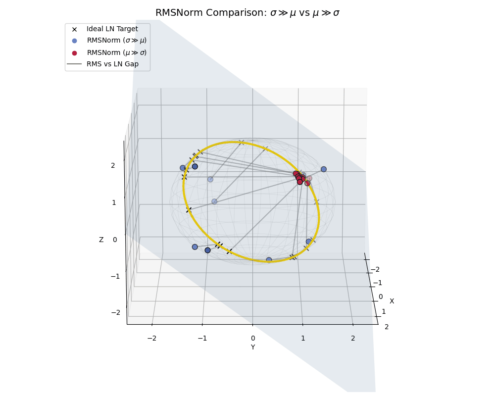A full comparison: High-variance data (blue) efficiently spreads out near the ideal LayerNorm equator, while low-variance, shifted data (crimson) is actively penalized and clustered near the poles.

Conclusion

By stripping away the algebra, we can see that normalization layers aren’t just statistical hacks; they are rigorous geometric constraints. They force chaotic, high-dimensional data to live on well-behaved, predictable manifolds ( spheres and ellipsoids ) so the subsequent attention layers can actually make sense of them.

RMSNorm’s success isn’t magic. It’s a calculated gamble that relies on the natural high-variance properties of deep neural networks to approximate the perfect spherical geometry of LayerNorm, while its built-in dampening ratio acts as a safety net when the model drifts.

That directional collapse has a practical implication worth sitting with. When a network goes unstable and activations spike ( the $\mu \gg \sigma$ regime ) standard LayerNorm silently corrects it by centering the data. RMSNorm doesn’t correct it; all tokens still land on the $\sqrt{n}$ sphere, but they pile up at one of two poles, becoming nearly indistinguishable from each other. The network doesn’t lose signal amplitude; it loses the ability to tell tokens apart. In most training runs this resolves itself because the gradient signal from the collapsed outputs steers the weights back toward the healthy regime. But it does suggest that RMSNorm models may be more sensitive to learning rate spikes and initialization choices that push mean activations far from zero early in training, a detail worth keeping in mind if you’re debugging a training instability.

More broadly, this geometric lens is a useful framework to carry forward. The next time you encounter a normalization variant ( RMSNorm with a learned offset, BatchNorm) you can ask the same questions: where does this operation constrain data to live, and what happens at the boundary conditions? The answer usually reveals both the method’s strengths and its failure modes far more clearly than the formula alone.

Code & Animations

The complete python script used to generate the 3D data, compute the projections, and render all the animations in this post is available in my repository.

Special thanks to Andy Arditi for his excellent research notes, and Paul M. Riechers for the formal geometric proofs.

---

If you have made it this far and found this article useful, you can buy me a bag of tea, it helps me keep writing posts like this one, as they’ve been taking more and more time :)) hopefully the quality shows off.